
Introduction to Deep Learning#
Warning
This chapter is by no means a complete introduction to deep learning. It is just a brief overview to refresh the main concepts.
Deep learning allows computational models that are composed of multiple processing layers to learn representations of data with multiple levels of abstraction. [LBH15]
What is Deep Learning?#
Deep Learning is a subfield of Machine Learning that involves the design, training, and evaluation of deep neural networks. While the term “deep” is not formally defined, it is generally used to refer to neural networks with more than one hidden layer.
What is a Neural Network?#
A neural network is a computational model inspired by the human brain. It is composed of a set of interconnected processing units, called neurons, that are organized in layers. Each neuron receives one or more inputs, performs a computation, and produces an output. The output of a neuron is then passed as input to other neurons. The output of the last layer is the output of the network.
The following figure shows a simple neural network with a single hidden layer. The network is composed of three layers:
input layer is the first layer of the network. It receives the input data and passes it to the next layer.
hidden layer is the middle layer of the network. It receives the input from the previous layer, performs a computation, and passes it to the next layer.
output layer is the last layer of the network. It receives the input from the previous layer, performs a computation, and produces the output of the network.
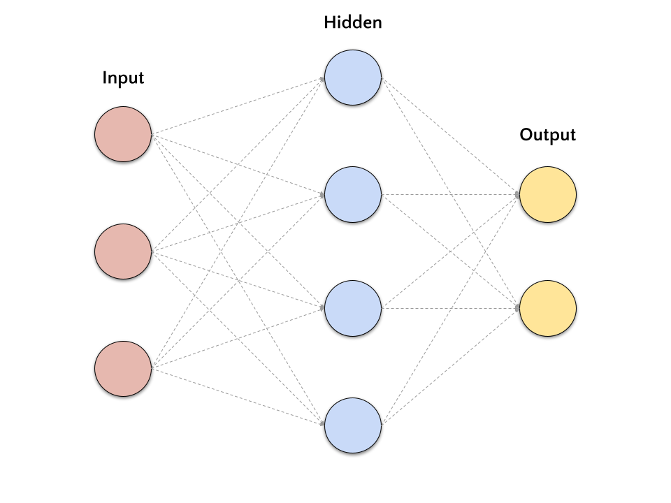
This kind of neural network is called feedforward neural network because the information flows from the input layer to the output layer without any feedback connections. Also, the network presented in the figure is called fully-connected neural network because each neuron in a layer is connected to all neurons in the next layer.
What is a Deep Neural Network?#
A deep neural network is a neural network with more than one hidden layer. The following figure shows a deep neural network with two hidden layers.
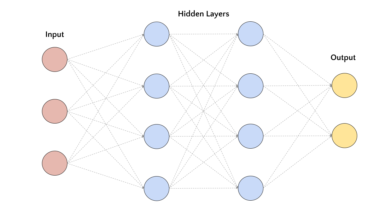
Similarly to the shallow case, the information flows from the input layer to the output layer without any feedback connections. Also, the network is fully-connected.
Exercise: How many connections?
What is the number of connections in a fully-connected neural network with \(n\) input neurons, \(m\) hidden neurons, and \(k\) output neurons?
The number of total connections is given by:
where \(l\) is the number of layers, \(n_i\) is the number of neurons in layer \(i\), and \(n_{i+1}\) is the number of neurons in layer \(i+1\).
What about the example in the figures above? How many connections are there in the shallow and deep neural networks?
Shallow neural network ( 3 - 4 - 2 ): \(3 \times 4 + 4 \times 2 = 20\)
Deep neural network ( 3 - 4 - 4 - 2 ): \(3 \times 4 + 4 \times 4 + 4 \times 2 = 36\)
Supervised Learning#
Deep learning models need to be trained on a collection of data to learn a specific task. The training process is based on the learning paradigm used to train the model. There are three main learning paradigms:
Supervised learning the training data is composed of input-output pairs. The goal of the model is to learn a function that maps the input to the output.
Unsupervised learning the training data is composed of input data only. The goal of the model is to learn the underlying structure of the data.
Reinforcement learning the training data is composed of input data and a reward signal. The goal of the model is to learn a policy that maximizes the reward.
Note
In this course we will focus on supervised learning, which is the most common learning paradigm in deep learning. While unsupervised and reinforcement learning are very important topics in deep learning, they are out of the scope of this course.
Supervised Learning (and self-supervised learning) is, at the moment, the most common learning paradigm in deep learning. The supervision is given by the training data, which is composed of input-output pairs. To formalize the problem, we can define the training data as a set of \(N\) input-output pairs:
where \(\mathbf{x}_i\) is the input and \(\mathbf{y}_i\) is the output for the \(i\)-th pair.
The goal of the model is to learn a function \(f\) that maps the input \(\mathbf{x}\) to the output \(\mathbf{y}\):
In the context of deep learning, the function \(f\) is implemented as a neural network.
Loss Function#
The training process consists in finding the parameters of the neural network that minimize a loss function \(\mathcal{L}\). It measures the difference between the predicted output \(\mathbf{\hat{y}}\) and the ground truth output \(\mathbf{y}\):
The loss function is a measure of how good the model is at predicting the output \(\mathbf{y}\) given the input \(\mathbf{x}\). The goal of the training process is to find the parameters of the neural network that minimize the loss function.
Some examples of loss functions are:
mean squared error \(\mathcal{L}(\mathbf{y}, \mathbf{\hat{y}}) = \frac{1}{N} \sum_{i=1}^N (\mathbf{y}_i - \mathbf{\hat{y}}_i)^2\). It is used for regression problems (e.g., predict a single real valued number - house price).
cross-entropy \(\mathcal{L}(\mathbf{y}, \mathbf{\hat{y}}) = - \sum_{i=1}^N \mathbf{y}_i \log(\mathbf{\hat{y}}_i)\). It is used for classification problems (e.g., predict a probability distribution over a set of classes - image classification).
Optimization#
A neural network is composed of neurons and connections between neurons. Each connection has a weight \(w_i\) that controls the information flow between neurons.
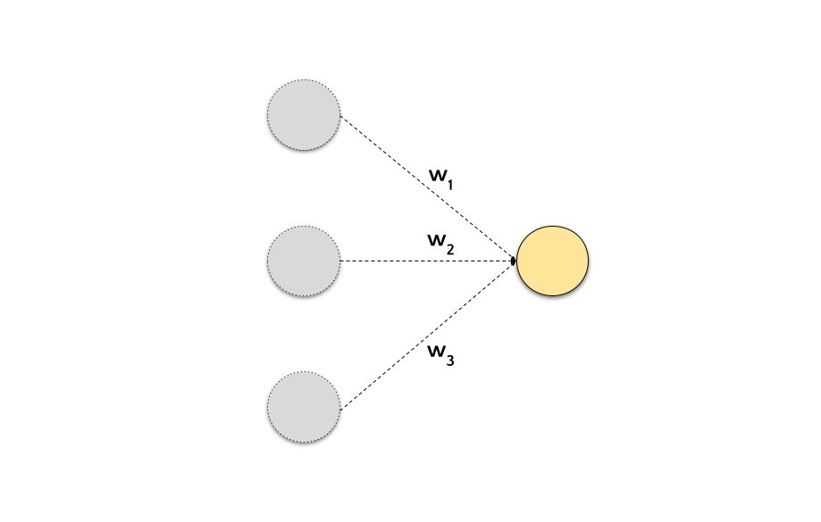
In the figure \(w_1, w_2, w_3\) are the weights of the connections between the preceding neurons and the current neuron. The weights are the parameters of the neural network. The goal of the training process is to find the optimal values for the weights that minimize the loss function.
Defined in this way, the neural network is a function \(f\) that maps the input \(\mathbf{x}\) to the output \(\mathbf{y}\) using a linear combination of the input and the weights:
However, in practice, we are interested in learning more complex functions. To this end, we need to introduce a non-linear activation function \(g\) that is applied to the output of each neuron:
The addition of a non-linear activation function introduces non-linearity to the model. This is essential because real-world data is often complex and non-linear. Without non-linear activation functions, the neural network would be limited to representing linear mappings, which are not sufficient for capturing intricate relationships in data.
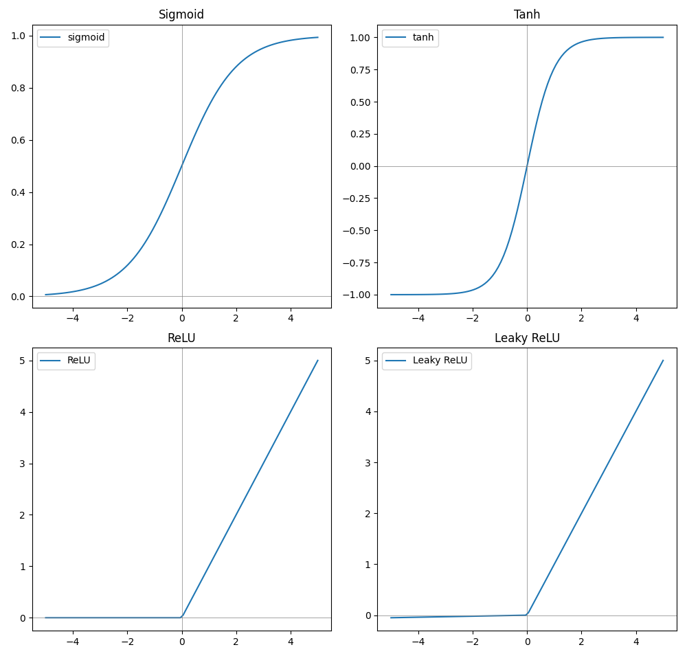
Some examples of activation functions are:
sigmoid \(g(x) = \frac{1}{1 + e^{-x}}\)
tanh \(g(x) = \frac{e^x - e^{-x}}{e^x + e^{-x}}\)
ReLU \(g(x) = \max(0, x)\)
Leaky ReLU \(g(x) = \max(0.01x, x)\)
Code: Activation Functions
The following code snippet draws the activation functions described above.
import matplotlib.pyplot as plt
import numpy as np

def sigmoid(x):
    return 1 / (1 + np.exp(-x))

def tanh(x):
    return (np.exp(x) - np.exp(-x)) / (np.exp(x) + np.exp(-x))

def relu(x):
    return np.maximum(0, x)

def leaky_relu(x):
    return np.maximum(0.01 * x, x)

x = np.linspace(-5, 5, 100)
y_sigmoid = sigmoid(x)
y_tanh = tanh(x)
y_relu = relu(x)
y_leaky_relu = leaky_relu(x)

# Create subplots
fig, axs = plt.subplots(2, 2, figsize=(10, 10))

# Plot sigmoid in the first subplot
axs[0, 0].plot(x, y_sigmoid, label='sigmoid')
axs[0, 0].set_title('Sigmoid')
axs[0, 0].axhline(0, color='gray', linewidth=0.5)
axs[0, 0].axvline(0, color='gray', linewidth=0.5)

# Plot tanh in the second subplot
axs[0, 1].plot(x, y_tanh, label='tanh')
axs[0, 1].set_title('Tanh')
axs[0, 1].axhline(0, color='gray', linewidth=0.5)
axs[0, 1].axvline(0, color='gray', linewidth=0.5)

# Plot ReLU in the third subplot
axs[1, 0].plot(x, y_relu, label='ReLU')
axs[1, 0].set_title('ReLU')
axs[1, 0].axhline(0, color='gray', linewidth=0.5)
axs[1, 0].axvline(0, color='gray', linewidth=0.5)

# Plot Leaky ReLU in the fourth subplot
axs[1, 1].plot(x, y_leaky_relu, label='Leaky ReLU')
axs[1, 1].set_title('Leaky ReLU')
axs[1, 1].axhline(0, color='gray', linewidth=0.5)
axs[1, 1].axvline(0, color='gray', linewidth=0.5)

# Add legend to each subplot
for ax in axs.flat:
    ax.legend()

# Adjust layout
plt.tight_layout()

# Save the figure
plt.savefig('activation_functions_subplots_with_axes.png')

# Show the plot
plt.show()
How to find the optimal values for the weights?
The training process is based on the gradient descent algorithm (or some variant of it). The gradient descent algorithm is an iterative algorithm that updates the weights of the neural network at each iteration. The update rule is the following:
where \(\alpha\) is the learning rate, which controls the size of the update. The learning rate is a hyperparameter of the model. The partial derivative \(\frac{\partial \mathcal{L}}{\partial w_i}\) is the gradient of the loss function with respect to the weight \(w_i\).
Backpropagation is an algorithm that computes the gradient of the loss function with respect to the weights of the neural network. It is based on the chain rule of calculus. The backpropagation algorithm is used to compute the gradient of the loss function with respect to the weights of the neural network.
The optimization process to train a neural network is the following:
Initialize the weights of the neural network
Forward propagation: compute the output of the neural network given the input \(\mathbf{x}\) and the weights \(\mathbf{w}\)
Compute the loss function \(\mathcal{L}(\mathbf{y}, \mathbf{\hat{y}})\)
Backward propagation: compute the gradient of the loss function with respect to the weights of the neural network
Update the weights of the neural network using the gradient descent algorithm
Repeat steps 2-5 until the loss function is minimized
The following figure shows the training process of a neural network. The training data is composed of input-output pairs. The neural network is initialized with random weights. The training process consists in updating the weights of the neural network to minimize the loss function.
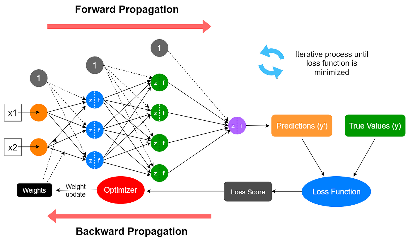
Fig. 2 Sketch of the training process of a neural network. Image from medium#
Activation Functions and Gradients#
The choice of the activation function is very important because it affects the training process. In particular, the activation function must be differentiable because we need to compute the gradient of the loss function with respect to the weights of the neural network.
Gradients of the loss function with respect to the weights are crucial for the backpropagation algorithm, which updates the weights in the direction that minimizes the loss. Therefore, the activation function must have the following properties:
Differentiability: the activation function must be differentiable for all values of its input.
Continuous gradients: the gradient of the activation function must be continuous for all values of its input. Continuous gradients facilitate stable weight updates during training.
Non-zero gradients: the gradient of the activation function must be non-zero for all values of its input.
Smoothness: the smoothness of the activation function allows consistent weight updates during training.
One problem during the training process is the vanishing gradient. The vanishing gradient problem occurs when the gradient of the activation function is close to zero. In this case, the weights are not updated during the training process. Similarly, the exploding gradient problem occurs when the gradient of the activation function is very large. In this case, the weights are updated too much during the training process. The choice of the activation function could mitigate those problems.
Optimization of a complex model#
In deep learning:
the neural network is composed of multiple layers
each layer is composed of multiple neurons
each neuron has multiple weights
The number of parameters in real-world neural networks grows very quickly. For this reason, while optimizing the parameters of a neural network, we usually parallelize the computation of the gradient. In other words, instead of having a single training example \(\mathbf{x_i}\), we use a batch of training examples \(\mathbf{X} = \{\mathbf{x_1}, \mathbf{x_2}, \dots, \mathbf{x_N}\}\) to compute the gradient. This approach is called mini-batch gradient descent. The size of the mini-batch \(N\) is a hyperparameter of the model.
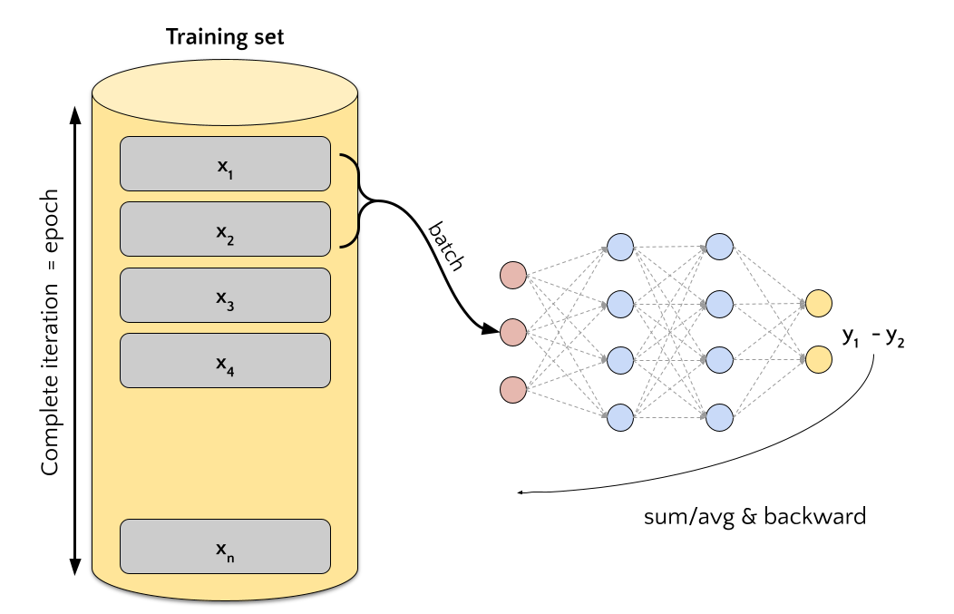
Fig. 3 Training process with mini-batch. A complete iteration over the training data is called epoch.#
Training and Validation#
The training process involves the definition of the following components:
neural network architecture
loss function
optimization algorithm
hyperparameters (e.g., learning rate, batch size, etc.)
dataset(s)
metrics to evaluate the model
In the superised learning setting, the training data is composed of input-output pairs. We are interested in training a model that is able to generalize to unseen data. To this end, we need to split the training data into (at least) two sets:
training set is used to train the model
test set is used to evaluate the model on unseen data
In principle, those two splits should be enough to train and evaluate the model. However, in practice, we need to tune the hyperparameters of the model. In other words, we need to find the best set of hyperparameters that minimize the loss function on the test set. To this end, we need to split the training set into two sets:
Training set is used to train the model.
validation set is used to evaluate the model during the training process (e.g., at each epoch) and it is used to tune the set of hyperparameters (e.g., the learning rate \(\alpha\), the number of epochs, etc.).
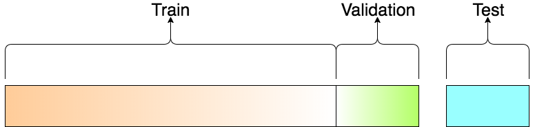
Fig. 4 Split of the training data into training, validation, and test sets. Image from towards data science#
Considering the data split, the training process now involves the following steps:
Split the training data into training, validation, and test sets.
Train the model on the training set.
Evaluate the model on the validation set.
Tune the hyperparameters of the model.
Repeat steps 2-4 until the final model is selected.
Evaluate the final model on the test set.
Note
In traditional machine learning is common to used cross-validation to tune the hyperparameters of the model. However, in deep learning, the training process is computationally expensive and the data is usually large. For this reason, we usually split the data into fixed training, validation, and test sets.
Code: Train-Validation-Test Split
The following code snippet shows how to split the data into training, validation, and test sets using scikit-learn.
from sklearn.model_selection import train_test_split

X, y = load_data() # Load the data

# split the data into training and test sets
X_train, X_test, y_train, y_test = train_test_split(X, y, test_size=0.2)
# split the training data into training and validation sets
X_train, X_val, y_train, y_val = train_test_split(X_train, y_train, test_size=0.2)
Evaluation Metrics#
The evaluation of a model is based on the evaluation metric(s). The evaluation metric is a function that measures the performance of the model on the test set. The choice of the evaluation metric depends on the task we are trying to solve.
Classification is the task of predicting a class label given an input. Some commonly used evaluation metrics for classification are:
accuracy is the ratio between the number of correct predictions and the total number of predictions. It is the most common evaluation metric for classification problems.
precision is the ratio between the number of true positives and the number of true positives and false positives. It measures the ability of the model to correctly predict the positive class.
recall is the ratio between the number of true positives and the number of true positives and false negatives. It measures the ability of the model to correctly predict the positive class.
F1-score is the harmonic mean of precision and recall. It is a single metric that combines precision and recall.
Many other evaluation metrics are available for classification problems. For example, the confusion matrix, the ROC curve, and the AUC are commonly used to evaluate classification models.
Regression is the task of predicting a real-valued number given an input. Some commonly used evaluation metrics for regression are:
mean squared error (MSE) is the average of the squared differences between the predicted value and the ground truth value. It is the most common evaluation metric for regression problems.
mean absolute error is the average of the absolute differences between the predicted value and the ground truth value.
root mean squared error (RMSE) is the square root of the average of the squared differences between the predicted value and the ground truth value.
Code: Evaluation Metrics
In python, there are different packages that implement the evaluation metrics described above. For example, scikit-learn supports many evaluation metrics for classification and regression problems.
from sklearn.metrics import accuracy_score, precision_score, recall_score, f1_score

y_true = [0, 1, 2, 0, 1, 2]
y_pred = [0, 2, 1, 0, 0, 1]

# Compute accuracy
accuracy = accuracy_score(y_true, y_pred)
precision = precision_score(y_true, y_pred, average='macro')
recall = recall_score(y_true, y_pred, average='macro')
f1 = f1_score(y_true, y_pred, average='macro')
print(f'Accuracy: {accuracy}')
print(f'Precision: {precision}')
print(f'Recall: {recall}')
print(f'F1-score: {f1}')
Many other evaluation metrics are available for regression problems. For example, the mean absolute percentage error (MAPE) is commonly used to evaluate regression models.
Conclusion#
In this chapter, we refreshed the main concepts of deep learning. In particular, we introduced the main components of a deep learning model and the training process. We also introduced the main evaluation metrics for classification and regression problems.
With this in mind, we are ready to deep dive into the architectures and applications of deep learning models for speech and vision.