Deep Learning Libraries#

Fig. 46 Image generated using OpenDALL-E#
In this chapter, we will see some some libraries that are useful to build, train and monitor deep learning models. More specifically, we will see:
PyTorch: a Python library that provides a wide range of tools to build and train deep learning models.
HuggingFace Transformers: Python library that provides access to pre-trained models for a variety of domains, including NLP, Computer Vision and Speech Processing.
Comet: an online platform that allows you to monitor specific metrics during training.
Learning Objectives
Understand the main concepts of PyTorch
Analyze the main features of HuggingFace Transformers and how to use them
How to monitor the training process to identify potential issues and understand the model behavior
During the exercises, you will be asked to implement specific components of common deep learning pipelines. You will be asked to use the libraries presented in this chapter. However, you are encouraged to use other libraries if you prefer. For the exercises, you can use the Google Colab environment. It is a free environment that allows you to run Python code in the cloud. It also provides free GPUs and TPUs. You can find more information here.
Deep learning libraries#
There are many deep learning libraries available. Some of them are more general, while others are more specific. In this section, we will see some of the most popular libraries.
PyTorch#
From a research perspective, PyTorch is one of the most popular deep learning libraries. It is a Python library that provides a wide range of tools to build and train deep learning models. It is also the library used in this book. PyTorch is based on the Torch library, which is a scientific computing framework with wide support for machine learning algorithms. PyTorch is developed by Facebook’s AI Research lab (FAIR) and since September 2022, it is a Linux Foundation project.
PyTorch is a Python library that allows you to build and train deep learning models. Some of the core concepts of PyTorch are:
Tensors: Tensors are the core data structure of PyTorch. They are similar to NumPy arrays, but they can be used on GPUs to accelerate computing.
Autograd: PyTorch provides automatic differentiation for all operations on Tensors. This means that you can compute gradients automatically. Namely, you can compute the gradients of the loss function with respect to the parameters of the model.
Neural networks: PyTorch provides a wide range of neural network layers and activation functions. It also provides a way to build neural networks using the
nn.Moduleclass (similarly to what we have seen in the previous chapters).Optimizers: PyTorch provides a wide range of optimizers, such as SGD, Adam, RMSProp, etc.
Data loaders: PyTorch provides a way to load data in batches. This is useful when you have a large dataset and you want to train your model on a GPU.
GPU support: PyTorch provides GPU support for all operations on Tensors. This means that you can train your model on a GPU and get faster results.
Distributed training: PyTorch provides a way to train your model on multiple GPUs or multiple machines. This is useful when you have a large dataset and you want to train your model on multiple GPUs or multiple machines.
Tensors#
A tensor is a generalization of vectors and matrices. A tensor is a multidimensional array. For example, a vector is a 1-dimensional tensor, a matrix is a 2-dimensional tensor, and a 3-dimensional tensor is a 3-dimensional array. In PyTorch, tensors are represented by the torch.Tensor class. The torch.Tensor class is similar to the NumPy ndarray class. However, the torch.Tensor class provides GPU support for all operations on tensors. This means that you can perform operations on tensors on a GPU and get faster results.
import torch

# Create a tensor
x = torch.tensor([[1, 2, 3], [4, 5, 6]])
# shape: (2, 3)
print(x.shape)
# dtype: torch.int64
print(x.dtype)
# device: cpu
print(x.device)

# Create a tensor on GPU
x = torch.tensor([[1, 2, 3], [4, 5, 6]], device='cuda') # you can use mps on modern MacBooks
# ...
Autograd#
When you train a deep learning model, you need to compute the gradients of the loss function with respect to the parameters of the model. This is called backpropagation. PyTorch provides automatic differentiation for all operations on tensors. What this means is that you can compute gradients automatically. For example, if you have a tensor x and you want to compute the gradients of the loss function with respect to x, you can do it with the following code:
import torch

# only complex or float tensors can have gradients
# requires_grad=True means that we want to compute gradients
x = torch.tensor([1, 2, 3], requires_grad=True, dtype=torch.float32)
y = x ** 2
z = y.sum()
z.backward() # compute gradients
print(x.grad) # gradients of z with respect to x
This is useful when you want to train a deep learning model. The gradients are computed automatically, so you don’t have to backpropagate them manually. Autograd works by keeping track of all operations on tensors. When you call backward() on a tensor, autograd computes the gradients of the loss function with respect to the tensor. This is done by using the chain rule.
Neural networks#
The torch.nn module provides a wide range of neural network layers and activation functions. Convolutional, Transformer, Pooling… layers are available.
One of the most important classes in the torch.nn module is the nn.Module class. This class is used to build neural networks. It provides a way to define the forward pass of the neural network. The forward pass is the process of computing the output of the neural network given an input. The nn.Module class also provides a way to define the backward pass of the neural network. The backward pass is the process of computing the gradients of the loss function with respect to the parameters of the neural network. In most cases, you don’t need to define the backward pass manually so you can inherit from the nn.Module class and define the forward pass only.
import torch
import torch.nn as nn

class MyModel(nn.Module):
    def __init__(self):
        super().__init__()
        self.linear = nn.Linear(10, 1)
        self.relu = nn.ReLU()

    def forward(self, x):
        x = self.linear(x)
        x = self.relu(x)
        return x
Optimizers and Schedulers#
The optimizer of a neural network is the algorithm that is used to update the parameters of the neural network. The most popular optimizer is the Stochastic Gradient Descent (SGD) optimizer. It is used to update the parameters of the neural network by computing the gradients of the loss function with respect to the parameters of the neural network and then updating the parameters of the neural network using the gradients. PyTorch provides a wide range of optimizers, such as SGD, Adam, AdamW, RMSProp, etc.
import torch
import torch.nn as nn

model = nn.Linear(10, 1)
optimizer = torch.optim.SGD(model.parameters(), lr=0.01)
The optimizer takes as input the parameters of the neural network and the learning rate. The learning rate is a hyperparameter that controls how much the parameters of the neural network are updated. Most of the times, however, you don’t want a constant learning rate. You want to adjust the learning rate during training. This is done by using a learning rate scheduler. PyTorch provides a wide range of learning rate schedulers, such as StepLR, MultiStepLR, ExponentialLR, etc. For example, if we want to decrease the learning rate by a factor of 0.1 every 10 epochs, we can do it with the following code:
import torch
import torch.nn as nn

model = nn.Linear(10, 1)
optimizer = torch.optim.SGD(model.parameters(), lr=0.01)
scheduler = torch.optim.lr_scheduler.StepLR(optimizer, step_size=10, gamma=0.1)
💡 When using optimizers and schedulers, it is important to include them in the training loop. Each object has a step() method that should be called after each batch. For example:
for epoch in range(epochs):
    for batch in data_loader:
        # ...
        loss.backward()
        optimizer.step()
        scheduler.step()
        optimizer.zero_grad()
❓ Why do we need to call optimizer.zero_grad() after each batch?
When we compute the gradients using loss.backward(), the gradients are accumulated in the parameters of the neural network. Those gradients are used in optimizer.step() to update the parameters of the neural network.
Next time we call loss.backward(), the gradients are accumulated in the parameters of the neural network again. This means that the gradients are accumulated over and over at each batch. This is not what we want. Instead, we want to compute the gradients for each batch and then update the parameters of the neural network. After that, we want to reset the gradients to zero so that the gradients are not accumulated over and over at each batch. This is done by calling optimizer.zero_grad().
Datasets and DataLoaders#
When training a deep learning model, you need to load the data to feed it to the model. In almost all cases, you don’t want to feed a single example to the model. Instead, you want to use a batch of examples. This is done by using data loaders. Dataset and DataLoader are two classes that allow data manipulation in PyTorch.
Detailed explainations of Dataset and DataLoader are available in the CNN chapter. Hereafter we provide a brief summary of the two classes.
The Dataset class is used to load the data from the dataset. It is designed to provide a way to load the data from the dataset and to transform the data. The DataLoader class is used to load the data from the Dataset class. It provides a unified interface to divide the data into batches and to load the data from the Dataset class.
Exercise, 30 min
Select a dataset that is useful for your research. If you don’t have a dataset, you can use the German Emotional-TTS dataset that contains 300 identical sentences spoken by a single speaker in 8 different emotions (2.400 recordings in total for 175 minutes of speech).
👀 Hint: You can download the folder by executing the following command in your terminal: wget https://www.openslr.org/resources/110/thorsten-emotional_v02.tgz
Create a Dataset class that loads the data from the dataset. Then, create a DataLoader class that loads the data from the Dataset class.
GPU support#
PyTorch provides GPU support for all operations on tensors. This means that you can perform operations on tensors on a GPU and get faster results. To use a GPU, you need to create a tensor on a GPU. This is done by using the device argument of the torch.tensor function. For example, if you want to create a tensor on a GPU, you can do it with the following code:
import torch

x = torch.tensor([1, 2, 3], device='cuda')
To benchmark the speed of a GPU we can run the following code:
import torch
import time
x = torch.randn(10000, 10000, device='cuda')
y = torch.randn(10000, 10000, device='cuda')
start = time.time()
for i in range(10):
    z = x @ y
end = time.time()

gpu_time = end - start
print(f"10 x GEMM on GPU: {gpu_time} seconds")

x = torch.randn(10000, 10000)
y = torch.randn(10000, 10000)
start = time.time()
for i in range(10):
    z = x @ y
end = time.time()
cpu_time = end - start
print(f"10 x GEMM on CPU: {cpu_time} seconds")

print(f"GPU speedup: {cpu_time / gpu_time}")
# GEMM stands for General Matrix Multiplication
PyTorch does not support only NVIDIA GPUs. It also supports modern MacBooks with Apple Silicon. You can use the device='mps' argument to use the Apple Silicon GPU.
Distributed training#
When dealing with large models and large datasets, it is often necessary to train the model on multiple GPUs. PyTorch provides a way to train your model on multiple GPUs. This is done by using the torch.nn.DataParallel class. This class allows you to train your model on multiple GPUs by splitting the batch into multiple batches and then computing the gradients on each GPU. For example, if you have a batch of size 64 and you want to train your model on 2 GPUs, you can do it with the following code:
import torch
import torch.nn as nn

# ... define model ...
if torch.cuda.device_count() > 1:
    device = torch.device('cuda')
    model = nn.DataParallel(model) # replicate model to multiple GPUs

# ... create data loader ...
for batch in data_loader:
    # device management will be done automatically
    input = batch['input'].to(device) # send input to GPU
    target = batch['target'].to(device)
    output = model(input)
    # ... compute loss ...
    loss.backward()
    optimizer.step()
    optimizer.zero_grad()

# save model
# without DataParallel
# torch.save(model.state_dict(), 'model.pt')
# with DataParallel
torch.save(model.module.state_dict(), 'model.pt')
PyTorch also provides a way to train your model on multiple machines (DDP). This is done by using the torch.nn.parallel.DistributedDataParallel class. This class allows you to train your model on a single machine with multiple GPUs or multiple machines with multiple GPUs. However, it requires more setup than the torch.nn.DataParallel class. For example, if you want to train your model on 2 machines with 2 GPUs each, you can do it with the following code:
import torch
import torch.nn as nn
import torch.distributed as dist
import torch.multiprocessing as mp

def main():
    # ... define model ...
    if torch.cuda.device_count() > 1:
        mp.spawn(train, nprocs=torch.cuda.device_count(), args=(model,))
    else:
        train(0, model)

def train(gpu, model):
    rank = gpu
    dist.init_process_group(backend='nccl', init_method='env://', world_size=4, rank=rank)
    torch.cuda.set_device(gpu)
    model = model.to(gpu)
    ddp_model = nn.parallel.DistributedDataParallel(model, device_ids=[gpu])
    # ... create data loader ...
    for batch in data_loader:
        input = batch['input'].to(gpu)
        target = batch['target'].to(gpu)
        output = ddp_model(input)
        # ... compute loss ...
        loss.backward()
        optimizer.step()
        optimizer.zero_grad()

if __name__ == '__main__':
    main()
The setup is more complicated than the torch.nn.DataParallel class because you need to initialize the process group and set the device manually. This process is designed for more advanced use-cases. If you are interested in distributed training, you may want to take a look at PyTorch Lightning, a library that both simplifies and extends PyTorch’s capabilities. PyTorch Lightning is beyond the scope of this book, and you can contact the teacher if you want to learn more about it.
HuggingFace Transformers#
HuggingFace Transformers is a Python library that provides state-of-the-art models for a variety of domains, including NLP, Computer Vision and Speech Processing. As can be inferred from the name, the library mostly include transformer-based models.
The library is built on top of PyTorch (with some models also implemented in TensorFlow and JAX) and provides a unified API to use the models. The library allows the use of pre-trained models that can be found on the Model Hub.
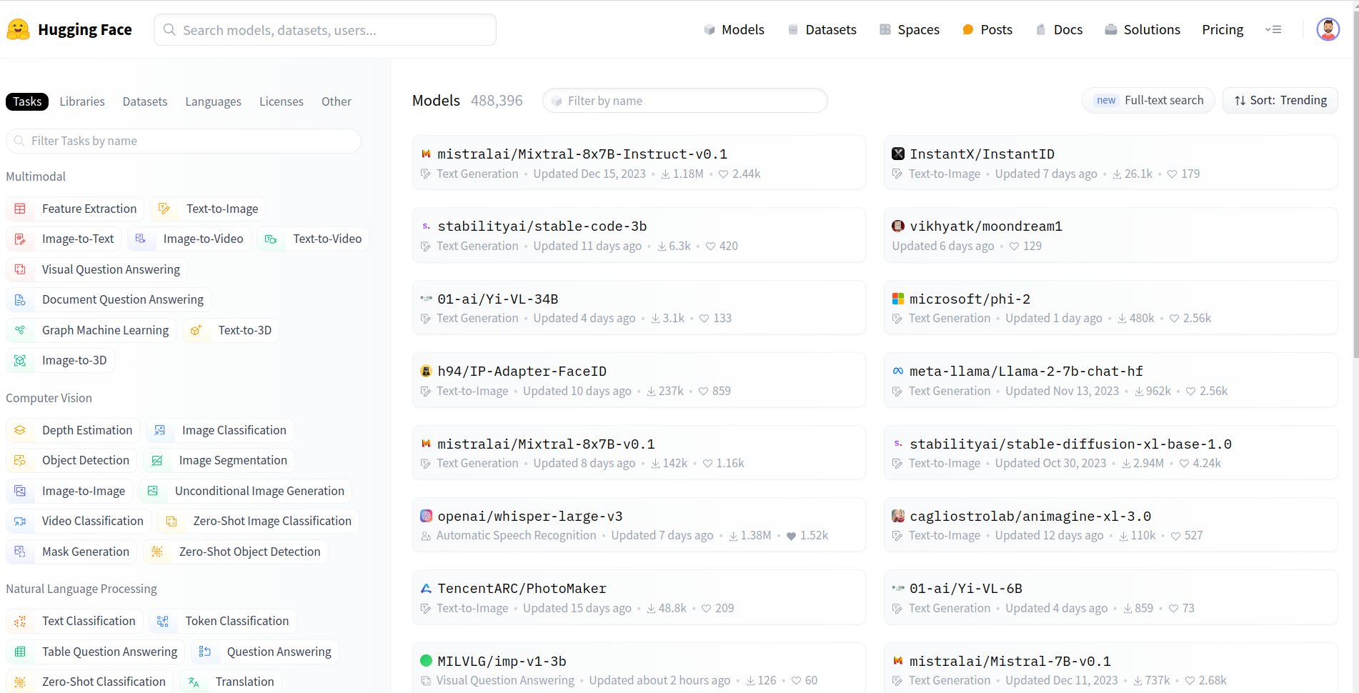
Fig. 47 Screenshot of the HuggingFace Model Hub#
As of January 2024, the hub includes almost 500.000 models (both pre-trained and fine-tuned) and is growing fast. It is possible to load pre-trained models, train new models, evaluate models and share models.
Depending on the model and the task, the library provides different classes and methods. However, the general workflow is the same for all models. The following code shows how to load a pre-trained model and use it to generate text:
import torch
from transformers import Wav2Vec2ForSequenceClassification, AutoFeatureExtractor

model_name = "facebook/wav2vec2-base" # identifier of the model
model = Wav2Vec2ForSequenceClassification.from_pretrained(model_name) # load the model
feature_extractor = AutoFeatureExtractor.from_pretrained(model_name) # load the feature extractor

sample_audio = torch.randn(16000) # 1 second of audio sampled at 16kHz
input_values = feature_extractor(sample_audio, sampling_rate=16000, return_tensors="pt").input_values # extract features

outputs = model(input_values) # forward pass
logits = outputs.logits # get logits
Most of the parameters are initialized by default, so it is suggested to carefully read the documentation of the model you want to use. For example, in the previous code, the classification head is initialized with 2 classes (positive and negative). If you want to use a different number of classes, you need to change the num_labels parameter.
import torch
from transformers import Wav2Vec2ForSequenceClassification, AutoFeatureExtractor

model_name = "facebook/wav2vec2-base" # identifier of the model
model = Wav2Vec2ForSequenceClassification.from_pretrained(model_name, num_labels=3) # load the model
feature_extractor = AutoFeatureExtractor.from_pretrained(model_name) # load the feature extractor

sample_audio = torch.randn(16000) # 1 second of audio sampled at 16kHz
input_values = feature_extractor(sample_audio, sampling_rate=16000, return_tensors="pt").input_values # extract features

outputs = model(input_values) # forward pass
logits = outputs.logits # get logits (shape: (1, 3))
Pre-trained models, in most cases, can be used as nn.Module objects. This means that you can use them in the same way you use PyTorch models. For example, you can train them using the nn.Module class and the torch.optim module.
import torch
from transformers import Wav2Vec2ForSequenceClassification, AutoFeatureExtractor

model_name = "facebook/wav2vec2-base" # identifier of the model
model = Wav2Vec2ForSequenceClassification.from_pretrained(model_name, num_labels=3) # load the model

# ... create data loader ...

optimizer = torch.optim.Adam(model.parameters(), lr=1e-4)
for batch in data_loader:
    input_values = batch['input_values']
    outputs = model(input_values) # forward pass
    loss = outputs.loss # get loss
    loss.backward() # compute gradients
    optimizer.step() # update parameters
    optimizer.zero_grad() # reset gradients
It is suggested to extract features in the __get_item__ method of the Dataset class, or in the data_collator of the DataLoader class. This is because the feature extraction is usually computationally expensive, thus parallelizing it is a good idea.
import torch
import torchaudio

class MyDataset(torch.utils.data.Dataset):
    def __init__(self, paths, labels):
        self.paths = paths
        self.labels = labels
        self.feature_extractor = AutoFeatureExtractor.from_pretrained("facebook/wav2vec2-base")

    def __getitem__(self, idx):
        path = self.paths[idx]
        label = self.labels[idx]
        audio, sr = torchaudio.load(path)
        # ... resample, normalize, etc ...
        features = self.feature_extractor(audio, sampling_rate=self.feature_extractor.sampling_rate, return_tensors="pt").input_values
        return {
            "input_values": features,
            "labels": label
        }
The library also provides a Trainer class that automate most of the training process. However, the simplicity comes at the cost of flexibility, thus to do non-standard training, it is suggested to implement the training loop manually. Using the trainer class is beyond the scope of this book, but you can find more information here.
Exercise, 40 min
Select a model from the Model Hub that is useful for your research. Use the Dataset you created in the previous exercise to fine-tune the model (e.g., for classification).
Implement a complete training setup, inclusing training, validation and testing. You can set standard parameters (e.g., batch size, learning rate, etc.) for educational purposes. However, you are encouraged to experiment with different parameters and to use a validation set to select the best model.
Model monitoring and visualization#
When training a deep learning model, it is important to monitor the training process. There exist many tools to monitor the training process:
… and many more
In this section, we will see how to use Comet to monitor the training process. It is an online platform that allows you to monitor specific metrics during training.
Comet#
To use Comet, you need to create an account on the website. Note: Comet is free for academic use. Once you have created an account, you can install the Python library by executing the following command in your terminal:
pip install comet-ml
Then, you can use the library to log metrics during training. For example, if you want to log the loss during training, you can do it with the following code:
from comet_ml import Experiment

# ... create model ...
experiment = Experiment(
    api_key="your_api_key",
    workspace="your_workspace",
    project_name="your_project_name"
)

for epoch in range(epochs):
    for batch in data_loader:
        # ... forward pass ...
        loss = ...
        experiment.log_metric("loss", loss)
Hereafter we explain each parameter of the Experiment class:
api_key: This is the API key that you can find on the website. You can also find it in the settings of your account.workspace: This is the name of your workspace. Usually, it is your username.project_name: This is the name of your project. If the project does not exist, it will be created automatically (e.g.,project_name="DL4SV-course").
⚠️ It is strongly suggested to not hard-code the API key in your code. Instead, you can use environment variables. For example, you can use the following code:
import os
from comet_ml import Experiment

experiment = Experiment(
    api_key=os.environ["COMET_API_KEY"],
    workspace=os.environ["COMET_WORKSPACE"],
    project_name="DL4SV-course"
)
To set the environment variables, you can use the following commands in your terminal:
export COMET_API_KEY="your_api_key"
export COMET_WORKSPACE="your_workspace"
or you can add them to your ~/.bashrc file to be loaded automatically at the lauch of a new terminal.
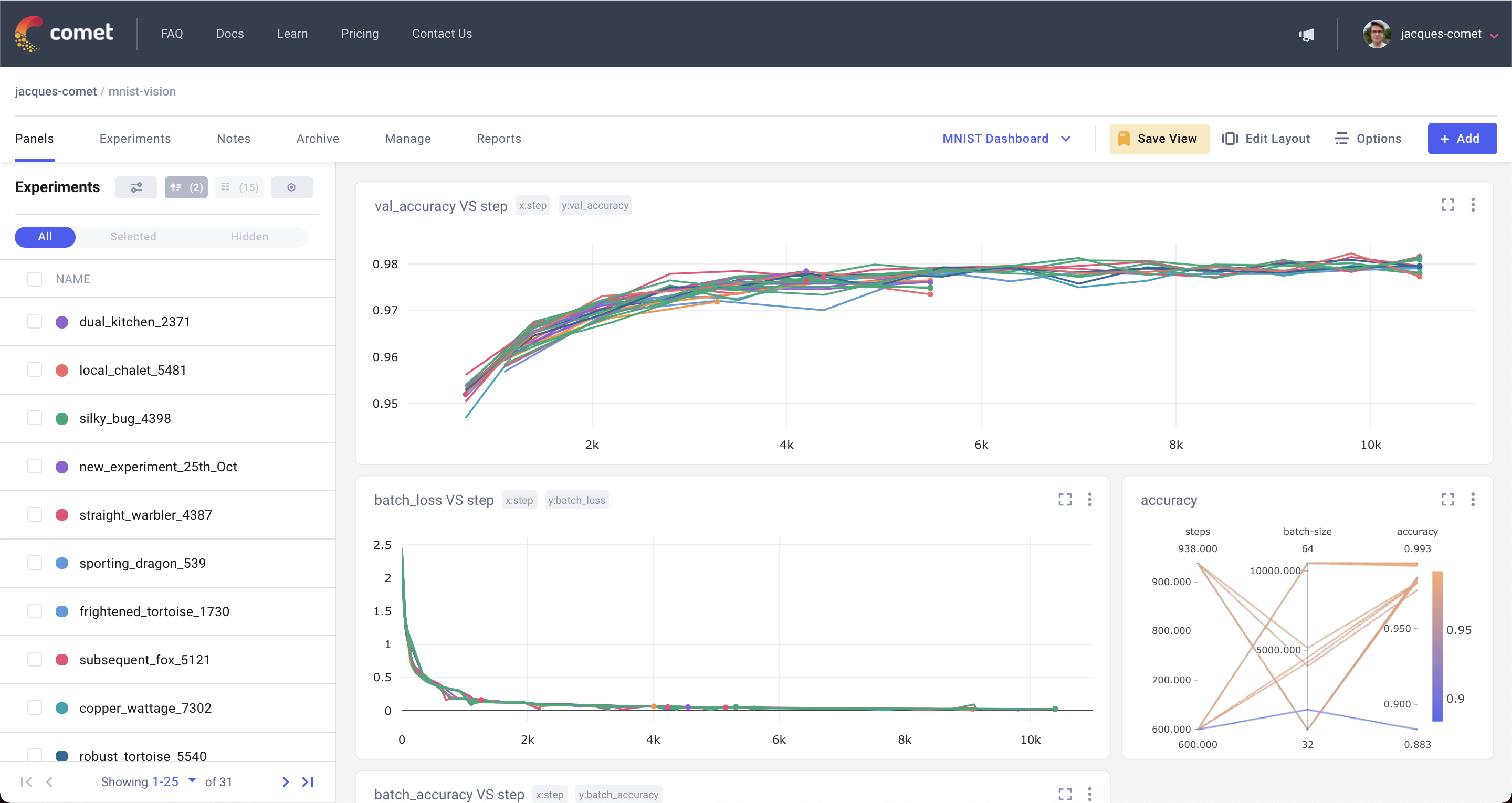
Once your training/evaluation is running, you can go to the website and see the metrics evolving in real-time.
There are additional and more advanced features that you can use. For example, you can log images, audio, text, etc. You can also log hyperparameters and tags. You can find more information here.
Exercise, 15 min
Modify the code of the previous exercise to log the loss during training. You can also log the validation loss and the accuracy.
Summary#
In this chapter, we have seen some of the most popular deep learning libraries. We have seen:
Libraries to build and train deep learning models - PyTorch in particular. It is the de-facto standard for research in computer vision, speech processing and many other domains.
Libraries to use pre-trained models - HuggingFace Transformers in particular. It allows to use pre-trained models in a simple and unified way. It focuses on transformer-based models, but it also includes other models.
Libraries to monitor the training process - Comet in particular. It allows to monitor specific metrics during training. It is free for academic use.
While this list is by no means exhaustive, it should give you a good starting point to create, manage and monitor your projects in the deep learning field. If you have specific requirements or you want to use a different library, you are encouraged to do so it by yourself or contact the teacher for more information.