Convolutional Neural Networks#

Fig. 5 Image generated using OpenDALL-E#
Introduction#
Convolutional Neural Networks (CNNs) are a class of deep neural networks that are widely used in computer vision applications. CNNs are designed to process data that have a grid-like or lattice-like topology, such as images, speech signals, and text.
The convolutional neural network architecture was first introduced in the 1980s by Yann LeCun and colleagues [LBD+89]. The first CNN was designed to recognize handwritten digits as the one shown in Figure The MNIST dataset . The network was trained on the MNIST dataset, a collection of 60000 handwritten digits.
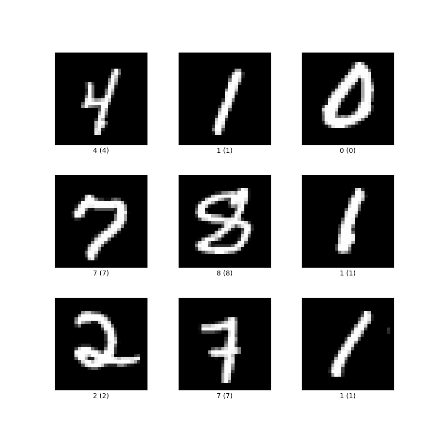
Fig. 6 The MNIST dataset#
Properties of Image Data#
Images are a special type of data that are characterized by three properties:
High dimensionality: images are represented as a matrix of pixels, where each pixel is a value between 0 and 255. For example, a 224x224 RGB image is represented as a 224x224x3 matrix (\(224 \times 224 \times 3 = 150528\)).
Spatial correlation: neaby pixel in an image are correlated. For example, in a picture of a cat, the pixels that represent the cat’s fur are likely to be similar.
Invariance to geometric transformations: the content of an image is invariant to geometric transformations such as translation, rotation, and scaling. For example, a picture of a cat is still a picture of a cat if we rotate it by 90 degrees.
Those properties are directly related to the fact that is really difficult to use a fully connected neural network to process images.
The high dimensionality of images makes the training of a fully connected neural network infeasible. Even a shallow network receiving as input a 224x224 RGB image would have 150528 input units in the first layer. This number would increase exponentially with the number of layers (2 layers \(150528^2\), 3 layers \(150528^3\), etc.).
The spatial correlation of images is not exploited by fully connected neural networks. In a fully connected neural network, each input unit is connected to each output unit. This means that the network would learn a different weight for each pixel in the image, regardless of its position. This is not desirable because the network would not be able to learn the spatial correlation between pixels.
Similarly, a fully connected neural network would not be able to learn the invariance to geometric transformations. If we translate, rotate, or scale an image, the network sees a completely different input.
Convolutional Neural Networks are designed to overcome these limitations.
Convolutional Neural Network Architecture#
The architecture of a convolutional neural network is composed of three main components:
Convolutional layers: these layers are responsible for extracting features from the input data. A convolutional layer is composed of a set of filters that are applied to the input data to extract features. The output of a convolutional layer is a set of feature maps, one for each filter.
Pooling layers: these layers are responsible for reducing the dimensionality of the feature maps. A pooling layer is applied to each feature map independently. Average or max pooling are the most common pooling strategies.
Fully connected layers: these layers are responsible for rearranging the features extracted by the convolutional layers into a vector of probabilities.
An example of a convolutional neural network architecture is shown in Figure Simple CNN architecture having all the basic components. Image source vitalflux.com. The network is composed of five convolutional layers, five pooling layers, and tthree fully connected layers. The input of the network is a 224x224 RGB image. The output of the network is a vector of probabilities, one for each class in the dataset (i.e., 1000 in the case of ImageNet).
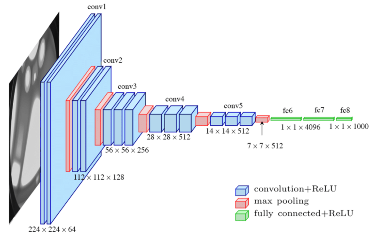
Fig. 7 Simple CNN architecture having all the basic components. Image source vitalflux.com#
The convolution operation, together with the pooling operation, is the key component of a convolutional neural network. In the following sections, we will see how these operations work and how they can be used to extract features from images.
Basic Components#
Convolutional neural networks, also named ConvNets or CNNs, are a class of deep neural networks that have been initially designed to process images. The operations involved in a CNN are inspired by the visual cortex of the human brain. In particular, the convolution operation is inspired by the receptive fields of neurons in the visual cortex.
Convolutional Layers#
The main component of a CNN is the convolutional layer. In a convolutional layer, a set of filters is applied to the input data to extract high-level features.
The convolution operation is defined by a set of parameters:
The filter size is the size of the filter. The filter size is usually an odd number (e.g., 3x3, 5x5, 7x7).
Stride is the number of pixels by which the filter is shifted at each step.
Padding is the number of pixels added to each side of the input image. Padding is usually used to preserve the spatial dimension of the input image.
The convolution operation is applied to each channel of the input image independently. For the moment, let’s consider a single channel image. The convolution operation is defined as follows:
The filter is placed on the top-left corner of the input image.
The element-wise multiplication between the filter and the input image is computed.
The result of the multiplication is summed up to obtain a single value.
The filter is shifted by the stride value to the right. If the filter reaches the right side of the image, it is shifted to the left side of the next row.
Steps 2-4 are repeated until the filter reaches the bottom-right corner of the image.
The result of the convolution operation is a feature map, a matrix of values that represents the output of the convolution operation.
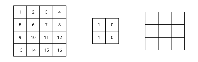
Fig. 8 Initial settings of the convolution operation. On the left, the input image. On the middle, the filter. On the right, the output feature map (empty at the beginning). In the example, stride is 1 and padding is 0 (simpler case).#
Fig. 8 shows the initial settings of the convolution operation. The feature map is empty at the beginning.
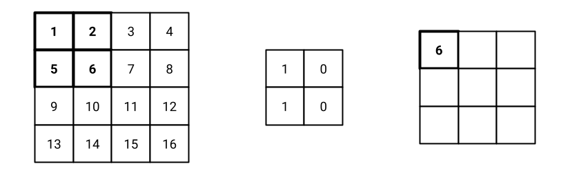
Fig. 9 Step 1 of the convolution operation.#
Step 1: the filter is placed on the top-left corner of the input image. The element-wise multiplication between the filter and the input image is computed. The result of the multiplication is summed up to obtain a single value. In this example, the result is 6, that is the first value of the feature map as shown in Fig. 9.
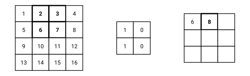
Fig. 10 Step 2 of the convolution operation.#
Step 2: the filter is shifted by the stride value to the right. If the filter reaches the right side of the image, it is shifted to the left side of the next row. In this example, the filter is shifted by 1 pixel to the right. The result of the convolution operation is 8, that is the second value of the feature map as shown in Fig. 10.
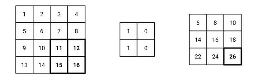
Fig. 11 Last step of the convolution operation.#
Step n: after \(n\) steps, the filter reaches the bottom-right corner of the image. The result of the convolution operation is a feature map, a matrix of values that represents the output of the convolution operation. In this example, the feature map is a 2x2 matrix as shown in Fig. 11.
The convolution operation is applied to each channel of the input image independently. The result is a set of feature maps, one for each channel of the input image. The number of feature maps is equal to the number of filters in the convolutional layer.
Note: in the previous example, we considered a fixed filter. In practice, the filters are learned during the training process. The weights of the filters are the parameters of the convolutional layer that the network learns during the training process.
Pooling Layers#
The pooling operation is often used to reduce the dimensionality of the feature maps. The pooling operation is defined by a set of parameters:
The pooling size is the size of the pooling filter. As for convolutional kernels, the pooling size is usually an odd number (e.g., 3x3, 5x5, 7x7).
Stride is the number of pixels by which the pooling filter is shifted at each step.
Padding is the number of pixels added to each side of the input image. Padding is usually used to preserve the spatial dimension of the input image.
Pooling strategy is the function used to aggregate the values in the pooling filter. The most common pooling strategies are average pooling and max pooling.
The pooling layer operates in a similar way to the convolutional layer. The pooling filter is placed on the top-left corner of the input image. The pooling operation is applied to each channel of the input image independently. The result of the pooling operation is a feature map, a matrix of values that represents the output of the pooling operation.
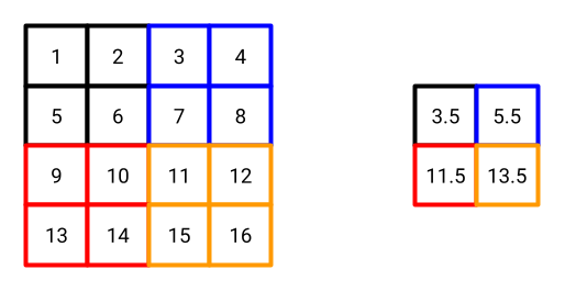
Fig. 12 Average pooling on a 4x4 matrix with pooling size 2x2 and stride 2. Padding is 0.#
Fig. 12 shows an example of average pooling. The colors help to visualize the pooling operation involving the following steps:
The pooling filter is placed on the top-left corner of the input image. The average of the values in the pooling filter is computed. In this example, the average is \((1+2+5+6)/4 = 3.5\).
The pooling filter is shifted by the stride value (2) to the right. Again, the average of the values in the pooling filter is computed. In this example, the average is \((3+4+7+8)/4 = 5.5\).
Since we reached the right side of the image, the pooling filter is shifted to the left side of the next row. The average of the values in the pooling filter is computed. In this example, the average is \((9+10+13+14)/4 = 11.5\).
… the process continues until the pooling filter reaches the bottom-right corner of the image.
Stride and Padding#
To this point, we have seen that the convolution and pooling operations are defined by a set of parameters. In particular, the stride and padding parameters are used to control the spatial dimension of the output feature maps.
Stride is the number of elements (pixels in an image) by which the filter is shifted at each step. The stride parameter is used to control the spatial dimension of the output feature maps. Common values for the stride parameter are 1 and 2. A stride of 1 means that the filter is shifted by 1 pixel at each step. A stride of 2 means that the filter is shifted by 2 pixels at each step.
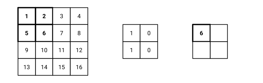
Fig. 13 Step 1 of the convolution operation with stride 2.#
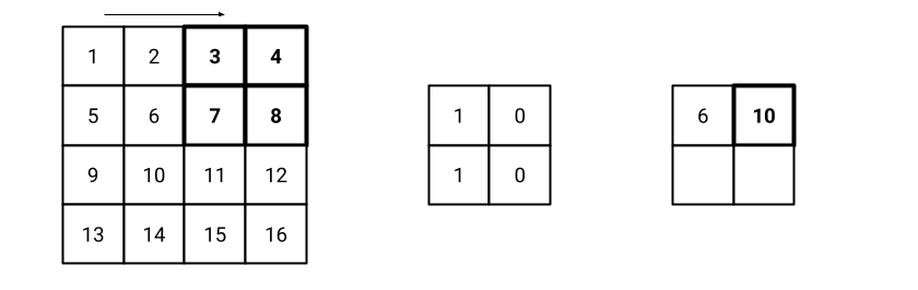
Fig. 14 Step 2 of the convolution operation with stride 2.#
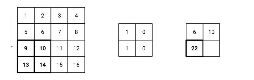
Fig. 15 Step 3 of the convolution operation with stride 2.#
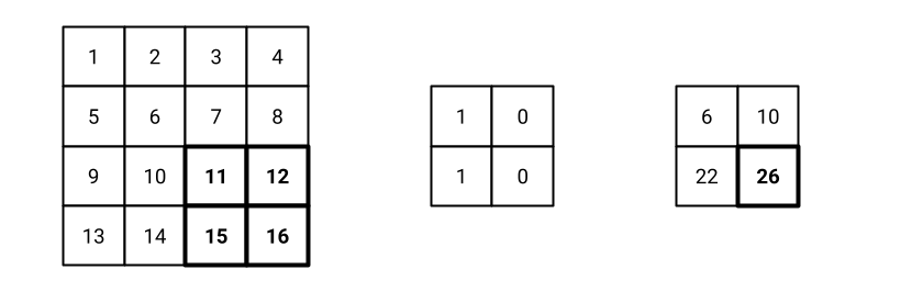
Fig. 16 Step 4 of the convolution operation with stride 2.#
Fig. 13 shows the initial settings of the convolution operation with stride 2. The filter is placed on the top-left corner of the input image. The result of the convolution operation is 6, that is the first value of the feature map. Similarly the process goes on until the filter reaches the bottom-right corner of the image. Fig. 14, Fig. 15, and Fig. 16 show the following steps of the convolution operation.
💡 Notice that the stride is the value by which the filter is shifted at each step both along the horizontal and vertical dimensions.
Padding is the number of elements (pixels in an image) added to each side of the input image. Padding is usually used to preserve the spatial dimension of the input image. In simple terms, padding is a “border” added to the input image. The value of the padding is usually 0 (zero padding - black border) or 1 (one padding - white border).
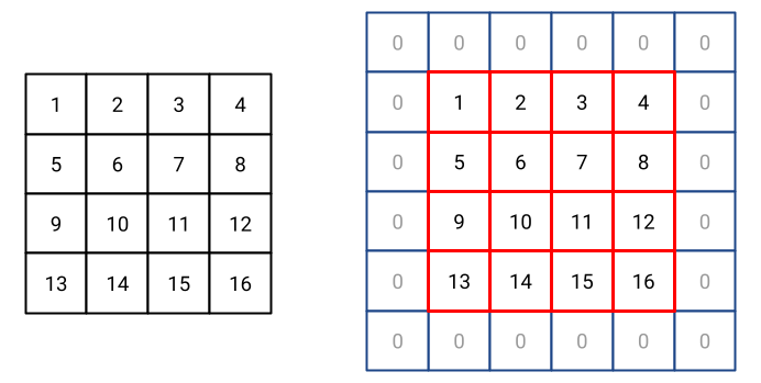
Fig. 17 Padding applied to a 4x4 matrix. Padding size is 1.#
Fig. 17 shows an example of padding. On the left, the input image. On the right, the padded image where the input matrix is reported in red and the padding is reported in blue. In this example, the padding size is 1. With an input image of size \(n \times n\), the output image has size \((n + 2p) \times (n + 2p)\), where \(p\) is the padding size. In the example of Fig. 17, the input image is a 4x4 matrix. The padding size is 1. The output image is a 6x6 matrix.
Computing the feature map size
Once set the parameters of the convolutional layer (filter size, stride, padding), it is possible to compute the size of the output feature map. The size of the output feature map is computed as follows:
For example, if the input image is a 224x224 RGB image, the filter size is 3x3, the stride is 1, and the padding is 0, the size of the output feature map is:
Intuitively, the output feature map is smaller than the input image because the filter cannot be placed on the edges of the image. The padding is used to preserve the spatial dimension of the input image (+ sign in the equation). The stride instead is used to control the reduction of the spatial dimension of the output feature map (i.e., the denominator of the equation).
Receptive Field#
One relevant concept in convolutional neural networks is the receptive field. It is defined as the portion of the input image that is visible to a single neuron in the network. The receptive field is usually defined in terms of the number of pixels in the input image. For example, a receptive field of 3x3 means that the neuron can “see” a 3x3 portion of the input image.
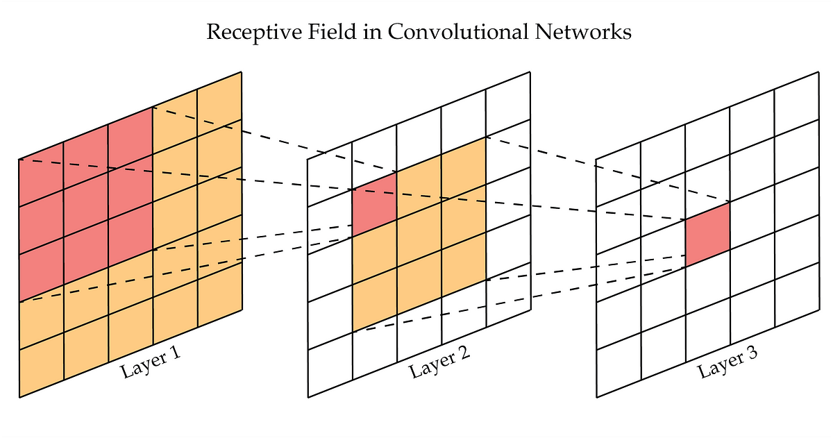
Fig. 18 Example of receptive field in a CNN.#
Fig. 18 shows an example of receptive field in a CNN. The receptive field of the neuron in the third layer is 3x3 when considering the second layer. If we consider the input image (e.g., layer 1), the receptive field of the same neuron would be 9x9 (the entire image is 5x5 so the neuron can “see” the whole image).
Intuitively, the receptive field defines the region of the input image that has contributed to the activation of a neuron in the network.
Common CNN Architectures#
Since the introduction of the first CNN architecture in the 1980s, many different architectures have been proposed. They differ in terms of the number of layers, the number of filters, the pooling strategy, etc., but also in terms of architectural choices that have been made to improve both the performance and the training process of the network.
LeNet-5#

Fig. 19 LeNet-5 architecture.#
LeNet-5 [LBD+89] is the first CNN architecture proposed by Yann LeCun and colleagues. The network was designed to recognize handwritten digits. The network is composed of 7 layers: 3 convolutional layers, 2 pooling layers, and 2 fully connected layers. The input of the network is a 32x32 grayscale image. The output of the network is a vector of probabilities, one for each class in the dataset (i.e., 10 in the case of MNIST).
We can see that since the first convolutional layer, the number of filters (number of channels in the feature maps) increases from 1 (greyscale image) to 6. On the other hand, the spatial dimension of the feature maps decreases from 32x32 to 28x28. This is one of the main characteristics shared by many CNN architectures: going deeper in the network, the number of filters increases while the spatial dimension of the feature maps decreases.
AlexNet#
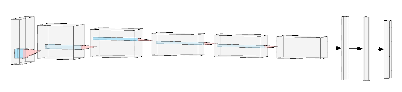
Fig. 20 AlexNet architecture.#
AlexNet [KSH12] is a CNN architecture proposed by Alex Krizhevsky and colleagues. The network was designed to classify images in the ImageNet dataset. The network is composed of 8 layers: 5 convolutional layers, 3 fully connected layers. The input of the network is a 224x224 RGB image. The output of the network is a vector of probabilities, one for each class in the dataset (i.e., 1000 in the case of ImageNet).
We can see that the network is composed of two groups of layers. The first group is composed of 5 convolutional layers and 3 pooling layers. The second group is composed of 3 fully connected layers. The first group is responsible for extracting features from the input image. The second group is responsible for classifying the input image.
It is worth mentioning that, at the time of its introduction, AlexNet was the first CNN architecture to use ReLU as activation function and dropout as regularization technique. AlexNet is also the winning entry of the ImageNet Large Scale Visual Recognition Challenge (ILSVRC) 2012, where it reduced the top-5 error by a large margin compared to the previous state-of-the-art.
ResNet#
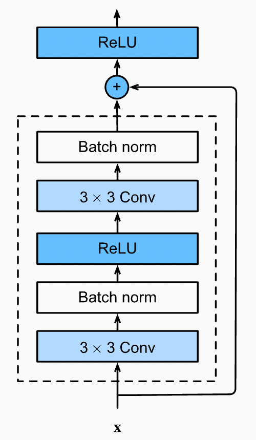
Fig. 21 ResBlock in ResNet architecture.#
ResNet [HZRS16a] is a CNN architecture proposed by Kaiming He and colleagues. Similarly to AlexNet, the network was designed to classify images in the ImageNet dataset. This network is the first to introduce the concept of residual learning that allows training very deep networks. There are different versions of ResNet, with 50, 101, 152, and 200 layers. The network is composed of a concatenation of residual blocks. Each residual block is composed of two convolutional layers, batch normalization, ReLU activation function, and a shortcut connection (i.e., the residual connection).
Fig. 21 shows an example of residual block. It is composed of two convolutional layers and a shortcut connection. The shortcut connection is used to add the input feature map to the output of the second convolutional layer. The output of the residual block is the sum of the input feature map and the output of the second convolutional layer. Batch normalization is applied after each convolutional layer and ReLU is used as activation function both after the first batch normalization and after the shortcut connection.
Residual Learning
Residual learning is a technique in training exceptionally deep neural networks. The fundamental concept involves incorporating a shortcut connection between the input and the output of a layer. Specifically, the output of the layer is formed by summing the input with the output of the layer.
The rationale behind residual learning lies in the belief that as layers are stacked in a network, the model can learn abstract features that are more useful for the downstream task than the shallower features acquired by less complex networks. However, this stacking of layers can bring to the vanishing gradient problem, a common obstacle in deep neural networks. The vanishing gradient problem manifests when the gradient of the loss function diminishes significantly with an increase in the number of layers. This slowdown in the gradient severely affect the training process.
Residual learning provides an elegant solution to the vanishing gradient problem by introducing a shortcut connection that directly links the input to the output of a layer. This shortcut connection facilitates an uninterrupted flow of the gradient from the output back to the input of the layer, effectively mitigating the challenges posed by the vanishing gradient problem. As a result, residual learning empowers the training of extremely deep networks, enabling them to capture intricate patterns and representations essential for complex tasks.
Fig. 22 Residual learning.#
Many other CNN architectures have been proposed in the last years. Here are some references if the reader is interested in learning more about CNN architectures:
VGG [SZ14], introduced the concept of using small convolutional filters (3x3) with stride 1 and padding 1.
DenseNet [HLVDMW17], introduced the concept of dense blocks, where each layer is connected to all the previous layers.
Inception [SLJ+15], introduced the concept of inception modules, where the input is processed by different convolutional filters and the output is concatenated.
MobileNet [HZC+17], introduced the concept of depthwise separable convolution, where the convolution operation is split into two separate operations: depthwise convolution and pointwise convolution.
EfficientNet [TL19], introduced the concept of compound scaling, where the depth, width, and resolution of the network are scaled together.
ConvNets for Audio Data#
The considerations made for image data are also valid for audio data. Audio data are characterized by high dimensionality and spatial correlation. For example, a 1-second audio clip sampled at 44.1 kHz is represented as a 44100-dimensional vector. Similarly to images, the use of standard fully connected neural networks is not feasible for audio data.
Exercise: FC for Audio Data
Consider a 1-second audio clip sampled at 44.1 kHz. The audio clip is represented as a 44100-dimensional vector. Suppose we want to use a fully connected neural network to classify the audio clip. The network is composed of 3 fully connected layers with 1000 units each. How many parameters does the network have?
The network has 45.1 million parameters. This is a huge number of parameters. Training such a network would require a lot of data and a lot of computational resources. Also, we are just considering a 1-second audio clip. In practice, audio clips used for classification tasks are usually longer than 1 second. For example, the audio clips in the AudioSet dataset are 10 seconds long, sampled at 16 kHz. This means that each audio clip is represented as a 160000-dimensional vector. The number of parameters of the network would increase exponentially.
1-D Convolutional Layers#
The convolution operation seen in the previous section can be applied to 1-dimensional data. In this case, the kernel is a 1-dimensional vector that slides along the input data. The output of the convolution operation is a 1-dimensional vector, the feature map.
The same concepts seen for 2-dimensional data are valid for 1-dimensional data. The convolution operation is defined by the same set of parameters: filter size, stride, and padding. The result is a set of feature maps, one for each channel of the input data.
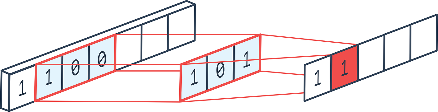
Fig. 23 1-D convolution.#
The convolution operation is applied to each channel of the input data independently. Similarly to the 2D-case, Convolutional Neural Networks are composed of a set of convolutional layers, pooling layers, and fully connected layers.
The main difference between 1D and 2D convolutional layers is that 1D convolutional layers are used to process 1-dimensional data (e.g., audio data) while 2D convolutional layers are used to process 2-dimensional data (e.g., image data).
💡 Note that, the number of channels and the number of dimensions are two different concepts. Dimensionality refers to the number of dimensions of the input data. Channels refers to the number of channels of the input data. For example, an audio clip recorded in stereo conditions (e.g., with two microphones) is a 1-dimensional signal with 2 channels. An audio clip recorded in mono conditions (e.g., with one microphone) is a 1-dimensional signal with 1 channel. Visual data usually have 3 channels (RGB images) and 2 dimensions (width and height).
Convolutional Layers for Temporal Patterns#
1D convolutional layers are usually used to extract temporal patterns from audio data. For example, a 1D convolutional layer can be used to extract the temporal patterns of a specific instrument in a music track.
Fig. 24 Example of 1D convolution with stride 1. Source: e2eml.school#

Fig. 25 Example of 1D convolution with stride 2. Source: e2eml.school#

Fig. 26 Example of 1D convolution with stride 4. Source: e2eml.school#
Fig. 24, Fig. 25, and Fig. 26 show an example of 1D convolution with stride 1, 2, and 4 respectively. The input data is a 1-dimensional vector of 25 elements. The filter is a 1-dimensional vector of 9 elements. The output of the convolution operation is a 1-dimensional vector of 16 elements. The number of elements in the output vector is computed as follows:
Multichannel 1D Convolution
One dimensional data may have multiple channels (e.g., stereo audio data). Similarly, an electroencephalograpy signal may come with 128 channels. A multichannel signal share a common dimension (e.g., the time axis) In this case each channel is processed independently by a 1D convolutional layer.
We should note that, we cannot expect that all data channels share the same temporal patterns. For example, in a stereo audio signal, the left and right channels may contain different instruments. For this reason, it is common to use a different set of filters for each channel.
Fig. 27 Example of multichannel 1D convolution. Source: e2eml.school#
Fig. 27 shows an example of multichannel 1D convolution. The input data is a 1-dimensional vector with 3 channels, we use 3 different filters to process each channel independently. The result of a multichannel convolution is a single channel output. Because the sliding dot product covers all the channels at once, they all get summed together and reduced down to a single channel. in-depth explanation
Spectrogram Representation#
Audio data are usually represented as a 1-dimensional vector that contains the amplitude of the signal at each time step.

Fig. 28 Example of audio waveform for a 30-second audio clip.#
Fig. 28 shows an example of audio waveform for a 30-second audio clip. The x-axis represents the time in seconds. The y-axis represents the amplitude of the signal. The audio clip is sampled at 16 kHz.
Note
How many samples are there in a 30-second audio clip sampled at 16 kHz?
However, the amplitude of the signal is not the only information that we can extract from an audio clip. For example, we can extract the frequency of the signal. The frequency of a signal is the number of cycles of a wave that occur in a second. The frequency of a signal is measured in Hertz (Hz). The frequency of a signal is related to the pitch of the sound. For example, a low-pitched sound has a low frequency while a high-pitched sound has a high frequency.
We can represent the frequency of a signal using a spectrogram. A spectrogram is a visual representation of the spectrum of frequencies of a signal as it varies with time. A spectrogram is usually represented as a 2-dimensional matrix where the x-axis represents the time in seconds and the y-axis represents the frequency in Hz. The color of each pixel represents the amplitude of the signal at a specific time and frequency bin.
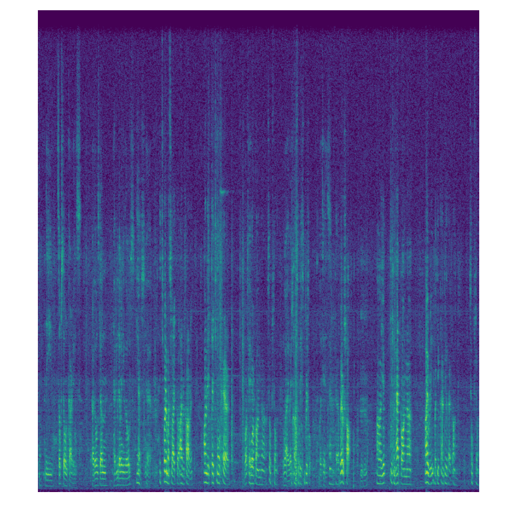
Fig. 29 Example of spectrogram for a 30-second audio clip.#
Fig. 29 shows an example of spectrogram for a 30-second audio clip. The x-axis represents the time in seconds. The y-axis represents the frequency in Hz. The color of each pixel represents the amplitude of the signal at a specific time and frequency bin.
Short-Time Fourier Transform#
The spectrogram is computed using the Short-Time Fourier Transform (STFT). The STFT is a technique to compute the Fourier transform of a signal over a short window of time. The Fourier transform is a mathematical operation that decomposes a signal into its constituent frequencies. The Fourier transform is defined as follows:
where \(x(t)\) is the signal, \(X(f)\) is the Fourier transform of the signal, and \(f\) is the frequency. However, the Fourier transform is defined for continuous signals. In practice, we usually deal with discrete signals. For this reason, we use the Discrete Fourier Transform (DFT) instead of the Fourier transform. The DFT is defined as follows:
where \(x(n)\) is the signal, \(X(k)\) is the DFT of the signal, \(k\) is the frequency, and \(N\) is the number of samples in the signal. The DFT is a discrete version of the Fourier transform.
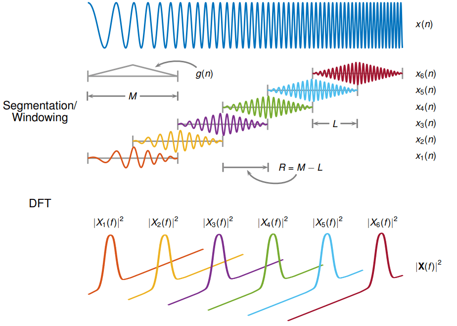
Fig. 30 Example of STFT process.#
Fig. 30 shows an example of STFT process. The input signal is a 1-dimensional vector (e.g., the audio file) represented as \(x(n)\). The STFT is computed by applying the DFT to a windowed portion of the signal. The window length in the image is \(M\) and the window shift is \(R\). \(L\) is the overlap between two consecutive windows. The output of the STFT is a 2-dimensional matrix (e.g., the spectrogram) represented as \(X(m, k)\).
Fig. 31 Example of STFT process in action.#
Fig. 31 shows an example of STFT process in action. The input signal is processed using a given window length and window shift. The output of the STFT is a 2-dimensional matrix (e.g., the spectrogram).
This section is not intended to be a comprehensive introduction to the STFT. For a more in-depth explanation, we refer the reader to specific online resources.
Mel-Spectrogram#
The spectrogram is a visual representation of the spectrum of frequencies of a signal as it varies with time. However, the human ear does not perceive all frequencies equally. For example, we are more sensitive to frequencies between 2 kHz and 5 kHz than to frequencies between 0 Hz and 1 kHz. For this reason, the spectrogram is usually converted into a Mel-spectrogram. A Mel-spectrogram is a spectrogram where the frequencies are converted into the Mel scale. The Mel scale is a perceptual scale of pitches judged by listeners to be equal in distance from one another. The Mel scale is defined as follows:
where \(f\) is the frequency in Hz and \(m\) is the frequency in Mel. The Mel scale is a non-linear transformation of the frequency scale. The Mel scale is used to convert the spectrogram into a Mel-spectrogram. The Mel-spectrogram is usually represented as a 2-dimensional matrix where the x-axis represents the time in seconds and the y-axis represents the frequency in Mel. The color of each pixel represents the amplitude of the signal at a specific time and frequency bin.
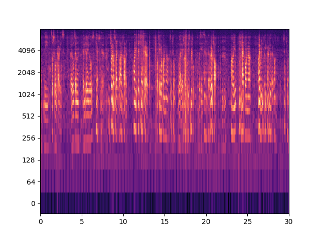
Fig. 32 Example of Mel-spectrogram for a 30-second audio clip.#
Fig. 32 shows an example of Mel-spectrogram for a 30-second audio clip. Mel-spectrogram is usually used as input to Convolutional Neural Networks for audio data. It is processed as a 2-dimensional image and similar architectures to those used for image data can be used.
Audio CNN Architectures#
Even if the concepts seen for image data are also valid for audio data, there are some differences between the two domains. For example, the receptive field of a neuron in a CNN for audio data may be much larger than the receptive field of a neuron in a CNN for image data. This is due to the fact that the temporal and spatial dimensions follow different rules and thus require different considerations.
Implementing a CNN with PyTorch#
PyTorch is an open source machine learning framework that accelerates the path from research prototyping to production deployment. PyTorch is developed by Facebook’s AI Research lab (FAIR) and is used in many research projects.
PyTorch is a Python package that allows the design of neural networks at both high and low levels. It offers different layers, optimizers, loss functions, etc. PyTorch also offers a set of tools to facilitate the training process of neural networks (e.g., data loaders, callbacks, etc.).
Dataset#
The Dataset class is an abstract class representing a dataset. The Dataset class is used to represent a collection of data samples. For example in supervised learning each sample is a pair (input, target). The input is the input data of the sample (e.g., an image, an audio clip, etc.). The target is the target data of the sample (e.g., a label, a class, etc.).
The Dataset class is an abstract class. This means that it cannot be instantiated directly. Instead, we need to create a subclass that inherits from the Dataset class. The subclass must implement two methods: __len__ and __getitem__. The __len__ method returns the size of the dataset. The __getitem__ method returns the sample at the given index.
from torch.utils.data import Dataset

class MyDataset(Dataset):
    def __init__(self, ...):
        # Initialize the dataset
        pass

    def __len__(self):
        # Return the size of the dataset
        pass

    def __getitem__(self, idx):
        # Return the sample at the given index
        pass
Specialized libraries exists in both Computer Vision and Audio Processing domains, torchvision and torchaudio. These libraries provide a set of datasets and utilities to facilitate the design of neural networks for Computer Vision and Audio Processing tasks.
MNIST#
The MNIST dataset is a dataset of handwritten digits. The dataset is composed of 60000 training samples and 10000 test samples. Each sample is a 28x28 grayscale image and the target is a digit between 0 and 9.
from torchvision.datasets import MNIST

# Download the dataset
train_dataset = MNIST(root="data/MNIST/", train=True, download=True)

# ! train_dataset is a Dataset object
# ! we do not need to implement the subclass

# Get the size of the dataset
print(len(train_dataset)) # 60000

# Get the sample at index 0
sample = train_dataset[0]
print(sample)
# (<PIL.Image.Image image mode=L size=28x28 at 0x7F9C70B726E0>, 5)
ITALian Intent Classification (ITALIC)#
The ITALIC dataset is a collection of around 16,000 audio recordings of Italian sentences. Each sentence has an associated intent, which is a label that describes the purpose of the sentence. The dataset is available on Zenodo. The dataset is also available through the huggingface datasets library.
This library provides a set of datasets that can be used for different tasks (e.g., image or audio classification).
from datasets import load_dataset

# Please be sure to use use_auth_token=True and to set the access token
# using huggingface-cli login
# or follow https://huggingface.co/docs/hub/security-tokens

# configs "hard_speaker" and "hard_noisy" are also available (to substitute "massive")
italic = load_dataset("RiTA-nlp/ITALIC", "massive", use_auth_token=True)
italic_train = italic["train"]
italic_valid = italic["validation"]
italic_test  = italic["test"]

# Get the size of the dataset
print(len(italic_train)) # 11514

# Get the sample at index 0
sample = italic_train[0]
print(sample)
# {'id': 1, 'age': 27, 'gender': 'male', 'region': 'abruzzo', 'nationality': 'italiana', 'lisp': 'nessuno', 'education': 'master', 'speaker_id': 72, 'environment': 'silent', 'device': 'phone', 'scenario': 'alarm', 'field': 'close', 'intent': 'alarm_set', 'utt': 'svegliami alle nove di mattina venerdì', 'audio': {'path': '/home/mlaquatra/.cache/huggingface/datasets/downloads/extracted/7f25fd6b6a74a983b3f0c3ea3ec3768f916c1fd6a84cd344bc1cedbd9249e698/zenodo_dataset/recordings/1.wav', 'array': array([0., 0., 0., ..., 0., 0., 0.], dtype=float32), 'sampling_rate': 16000}}
Dataset objects contain a convenient way to access the data. Also a Dataset class has the flexibility to provide different views of the data. If the model we are implementing requires a specific format for the data, we can implement a __getitem__ method that returns the data in the required format.
For example, we can implement a PyTorch Dataset class for the ITALIC dataset that returns a tuple or a dictionary containing the audio data and the target data.
from torch.utils.data import Dataset
from datasets import load_dataset

class ITALICDataset(Dataset):
    def __init__(self, split="train", format="tuple"):
        # Load the dataset
        self.dataset = load_dataset("RiTA-nlp/ITALIC", split, use_auth_token=True)
        self.format = format

    def __len__(self):
        # Return the size of the dataset
        return len(self.dataset)

    def __getitem__(self, idx):
        # Return the sample at the given index
        sample = self.dataset[idx]
        # Get the audio data
        audio = sample["audio"]["array"]
        # Get the target data
        target = sample["intent"]
        if self.format == "tuple":
            return audio, target
        elif self.format == "dict":
            return {"audio": audio, "target": target}
        else:
            raise ValueError("Format not supported")

train_dataset = ITALICDataset(split="train")
DataLoader#
Once we have defined a Dataset class, we can use it to create a DataLoader object. As we have seen in previous chapters, the training of a complex neural network requires the generation of batches of data. The DataLoader class is used to generate batches of data from a Dataset object.
from torch.utils.data import DataLoader

# Create a DataLoader object
train_dataloader = DataLoader(train_dataset, batch_size=32, shuffle=True)

# Iterate over the batches
for batch in train_dataloader:
    # Get the input data
    input_data = batch[0]
    # Get the target data
    target = batch[1]
    # Do something with the data
    pass
Depending on the split of data (e.g., train, validation, test), we can create different DataLoader objects. This is useful because, for training, we usually want to shuffle the data while for validation and test we do not want to shuffle the data.
from torch.utils.data import DataLoader

# Create a DataLoader object for training
train_dataloader = DataLoader(train_dataset, batch_size=32, shuffle=True)
# Create a DataLoader object for validation
valid_dataloader = DataLoader(valid_dataset, batch_size=32, shuffle=False)
...
The mix of Dataset and DataLoader classes is a powerful tool to manage the data in a machine learning project. The Dataset class is used to represent a collection of data samples. The DataLoader class is used to generate batches of data from a Dataset object.
Model#
The nn module [ref] provides a set of tools to design neural networks. The nn.Module class is an abstract class representing a neural network. It is used to represent a neural network. The nn.Module class is an abstract class. This means that it cannot be instantiated directly. Instead, we need to create a subclass that inherits from the nn.Module class.
Similar to the Dataset class, the subclass must implement two methods: __init__ and forward. The __init__ method is used to initialize the layers of the network. The forward method is used to define the forward pass of the network.
💡 Note that, the forward pass of the network is defined by the forward method. The backward pass is automatically computed by PyTorch using the autograd module.
import torch.nn as nn

class MyModel(nn.Module):
    def __init__(self, ...):
        # Initialize the layers of the network
        pass

    def forward(self, x):
        # Define the forward pass of the network
        pass
Convolutional Layers#
The nn module provides a set of layers that can be used to design a neural network. For example, the nn.Conv2d layer is used to implement a 2-dimensional convolutional layer. The nn.Conv1d layer is used to implement a 1-dimensional convolutional layer. The nn.Linear layer is used to implement a fully connected layer.
import torch.nn as nn

# 2D convolutional layer
conv2d = nn.Conv2d(in_channels=3, out_channels=16, kernel_size=3, stride=1, padding=1)

# 1D convolutional layer
conv1d = nn.Conv1d(in_channels=1, out_channels=16, kernel_size=3, stride=1, padding=1)

# Fully connected layer
linear = nn.Linear(in_features=1000, out_features=10)
Activation Functions#
The nn module also provides a set of activation functions that can be used to design a neural network. For example, the nn.ReLU layer is used to implement the ReLU activation function. The nn.Sigmoid layer is used to implement the Sigmoid activation function. The nn.Tanh layer is used to implement the Tanh activation function. The nn.Softmax layer is used to implement the Softmax activation function.
import torch.nn as nn

# ReLU activation function
relu = nn.ReLU()

# Sigmoid activation function
sigmoid = nn.Sigmoid()

# Tanh activation function
tanh = nn.Tanh()

...
Similarly, there exist other layers already implemented in PyTorch.
Pooling layers:
nn.MaxPool2d,nn.MaxPool1d,nn.AvgPool2d,nn.AvgPool1dNormalization layers:
nn.BatchNorm2d,nn.BatchNorm1dDropout layers:
nn.Dropout2d,nn.Dropout1dEmbedding layers:
nn.Embedding…
Loss Functions#
The nn module also provides a set of loss functions that can be used to design a neural network. For example, the nn.CrossEntropyLoss layer is used to implement the Cross Entropy loss function that is the standard loss function for classification tasks. The nn.MSELoss layer is used to implement the Mean Squared Error loss function that is the standard loss function for regression tasks.
import torch
import torch.nn as nn

predicitons = torch.randn(10, 5) # 10 samples, 5 classes
targets = torch.randn(10, 5) # 10 samples, 5 classes

# Cross Entropy loss function
loss_fn = nn.CrossEntropyLoss()
loss = loss_fn(predicitons, targets)
Optimizers and Schedulers#
When training our model, we need to define an optimizer and a scheduler.
The optimizer is used to update the parameters of the network. The optimizer is defined by the torch.optim module [ref]. The torch.optim module provides a set of optimizers that can be used to train a neural network. For example, the torch.optim.SGD optimizer is used to implement the Stochastic Gradient Descent optimizer. The torch.optim.Adam optimizer is used to implement the Adam optimizer.
import torch.optim as optim

# Stochastic Gradient Descent optimizer
optimizer = optim.SGD(model.parameters(), lr=0.01, momentum=0.9)
The scheduler is used to update the learning rate of the optimizer. Usually, we don’t want to use a fixed learning rate. Instead, we want to decrease the learning rate during the training process. The scheduler is defined by the torch.optim.lr_scheduler module [ref]. The torch.optim.lr_scheduler module provides a set of schedulers that can be used to train a neural network. For example, the torch.optim.lr_scheduler.StepLR scheduler is used to implement the StepLR scheduler. The torch.optim.lr_scheduler.ReduceLROnPlateau scheduler is used to implement the ReduceLROnPlateau scheduler.
import torch.optim as optim

# StepLR scheduler
scheduler = optim.lr_scheduler.StepLR(optimizer, step_size=30, gamma=0.1)
Training#
The training process of a neural network is usually composed of the following steps:
Forward pass: the input data is processed by the network to obtain the output data.
Loss computation: the output data is compared with the target data to compute the loss.
Backward pass: the loss is used to compute the gradients of the network parameters.
Parameters update: the gradients are used to update the parameters of the network.
# Iterate over the batches

model = model.train() # Set the model in training mode
# Why?

for batch in train_dataloader:
    # Get the input data
    input_data = batch[0]
    # Get the target data
    target = batch[1]
    # Forward pass
    output = model(input_data)
    # Loss computation
    loss = loss_fn(output, target)
    # Backward pass
    loss.backward()
    # Parameters update
    optimizer.step()
    # Reset the gradients
    optimizer.zero_grad()
💡 The optimizer.zero_grad() method is used to reset the gradients of the network parameters. This is necessary because PyTorch accumulates the gradients on subsequent backward passes. This means that, if we do not reset the gradients, the gradients will be accumulated on subsequent backward passes.
💡 The optimizer.step() method is used to update the parameters of the network. This is necessary because PyTorch does not update the parameters automatically. This means that, if we do not update the parameters, the parameters will not be updated.
💡 The loss.backward() method is used to backpropagate the loss. This step is basically performing the backward pass of the network.
Evaluation#
Once we have trained our model, we need to evaluate its performance on the test set. The evaluation process is similar to the training process. The main difference is that we do not need to update the parameters of the network.
model = model.eval() # Set the model in evaluation mode
# Why?
with torch.no_grad(): # Disable gradient computation
    for batch in test_dataloader:
        # Get the input data
        input_data = batch[0]
        # Get the target data
        target = batch[1]
        # Forward pass
        output = model(input_data)
        # Loss computation
        loss = loss_fn(output, target)
In this case, during evaluation we need to disable the gradient computation. This is necessary because we do not need to update the parameters of the network. If we do not disable the gradient computation, PyTorch will compute the gradients of the network parameters. This is not necessary during evaluation and it is a waste of computational resources.
💡 We did not use any specific metric to evaluate the performance of the model, we only computed the loss. However, in practice, we usually use different metrics to evaluate the performance of the model. For example, in classification tasks, we usually use the accuracy metric. In regression tasks, we usually use the mean squared error metric. Those metrics can be implemented saving the predictions and the targets and then computing the metric on the whole dataset.
predictions = []
targets = []

with torch.no_grad(): # Disable gradient computation
    for batch in test_dataloader:
        # Get the input data
        input_data = batch[0]
        # Get the target data
        target = batch[1]
        # Forward pass
        output = model(input_data)
        # Save the predictions
        predictions.append(output)
        # Save the targets
        targets.append(target)

# Concatenate the predictions
predictions = torch.cat(predictions, dim=0)
# Concatenate the targets
targets = torch.cat(targets, dim=0)

# Compute the accuracy
accuracy = (predictions.argmax(dim=1) == targets).float().mean()
Training My (First) CNN#
In this section, we will implement a simple CNN for the MNIST dataset. The MNIST dataset is a dataset of handwritten digits. The dataset is composed of 60000 training samples and 10000 test samples. Each sample is a 28x28 grayscale image and the target is a digit between 0 and 9.
import torch
import torch.nn as nn
import torch.optim as optim
from torch.utils.data import DataLoader
from torchvision.datasets import MNIST
from torchvision.transforms import ToTensor
from tqdm import tqdm # Progress bar

# Create the dataset
train_dataset = MNIST(root="data/MNIST/", train=True, download=True, transform=ToTensor())
test_dataset = MNIST(root="data/MNIST/", train=False, download=True, transform=ToTensor())

# we can implement a validation split, how?

# Create the dataloader
train_dataloader = DataLoader(train_dataset, batch_size=32, shuffle=True)
test_dataloader = DataLoader(test_dataset, batch_size=32, shuffle=False)

# Define the model
class MyModel(nn.Module):
    def __init__(self):
        super().__init__()
        self.conv1 = nn.Conv2d(in_channels=1, out_channels=16, kernel_size=3, stride=1, padding=1)
        self.relu1 = nn.ReLU()
        self.pool1 = nn.MaxPool2d(kernel_size=2, stride=2)
        self.conv2 = nn.Conv2d(in_channels=16, out_channels=32, kernel_size=3, stride=1, padding=1)
        self.relu2 = nn.ReLU()
        self.pool2 = nn.MaxPool2d(kernel_size=2, stride=2)
        self.linear1 = nn.Linear(in_features=32*7*7, out_features=10)

    def forward(self, x):
        x = self.conv1(x)
        x = self.relu1(x)
        x = self.pool1(x)
        x = self.conv2(x)
        x = self.relu2(x)
        x = self.pool2(x)
        x = x.view(x.size(0), -1)
        x = self.linear1(x)
        return x

# Create the model
model = MyModel()

# Define the loss function
loss_fn = nn.CrossEntropyLoss()

# Define the optimizer
optimizer = optim.SGD(model.parameters(), lr=0.01, momentum=0.9)
# Define the scheduler
scheduler = optim.lr_scheduler.StepLR(optimizer, step_size=30, gamma=0.1)

# Training loop
model = model.train() # Set the model in training mode
for epoch in range(10):
    # Iterate over the batches
    for batch in tqdm(train_dataloader):
        # Get the input data
        input_data = batch[0]
        # Get the target data
        target = batch[1]
        # Forward pass
        output = model(input_data)
        # Loss computation
        loss = loss_fn(output, target)
        # Backward pass
        loss.backward()
        # Parameters update
        optimizer.step()
        # Reset the gradients
        optimizer.zero_grad()
    # Update the learning rate
    scheduler.step()

# Evaluation loop
model = model.eval() # Set the model in evaluation mode

predictions = []
targets = []
with torch.no_grad(): # Disable gradient computation
    for batch in test_dataloader:
        # Get the input data
        input_data = batch[0]
        # Get the target data
        target = batch[1]
        # Forward pass
        output = model(input_data)
        # Save the predictions
        predictions.append(output)
        # Save the targets
        targets.append(target)

# Concatenate the predictions
predictions = torch.cat(predictions, dim=0)
# Concatenate the targets
targets = torch.cat(targets, dim=0)

# Compute the accuracy
accuracy = (predictions.argmax(dim=1) == targets).float().mean()
print(f"Accuracy: {accuracy:.2f}")
Assignment#
Implement a CNN for the ITALIC dataset. The ITALIC dataset is a collection of around 16,000 audio recordings of Italian sentences. The intent is a label that describes the purpose of the sentence.
Implement a complete pipeline to train and evaluate a CNN for Intent Classification. The pipeline should include the following steps:
Data loading: load the dataset.
Data preprocessing: preprocess the dataset when and if necessary.
Model definition: define the model architecture (you can use a 2D CNN if working with spectrograms or a 1D CNN if working with raw audio).
Model training: train the model - include a validation split and select the best model based on the validation performance.
Model evaluation: evaluate the model - compute specific metrics (e.g., accuracy).