Transformers#
Fig. 33 Image generated using OpenDALL-E#
Introduction#
In this chapter, we will cover the basics of transformers, a type of neural network architecture that has been initially developed for natural language processing (NLP) tasks but has since been used and adapted for other modalities such as images, audio, and video.
The transformer architecture is designed for modeling sequential data, such as text, audio, and video. It is based on the idea of self-attention, which is a mechanism that allows the network to learn the relationships between different elements of a sequence. For example, in the case of an audio sequence, the network can learn the relationships between different frames of the audio signal and leverage the correlations between them to perform a task such as speech recognition.
The original Transformer architecture was introduced in the paper Attention Is All You Need [VSP+17] by Vaswani et al. in 2017. Since then, many variants of the original architecture have been proposed, and transformers have become the state-of-the-art architecture for many tasks. In this chapter, we will cover all the building blocks of the transformer architecture and show how they can be used for different tasks.
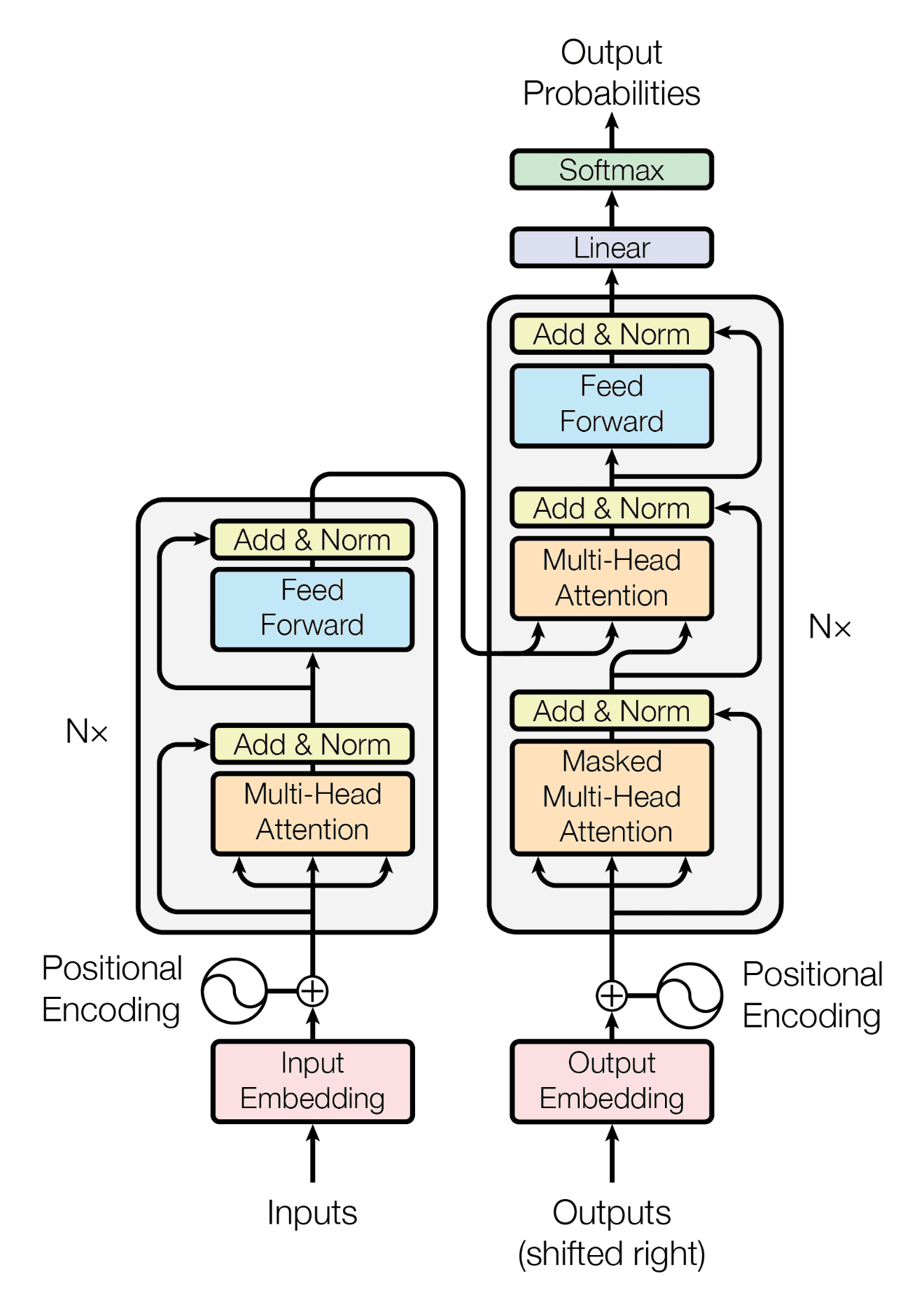
Fig. 34 Transformer architecture#
Architecture Overview#
Fig. 34 shows the architecture of the transformer model. The model consists of an encoder and a decoder.
The encoder is responsible for processing the input sequence and extracting relevant information.
The decoder is responsible for generating the output sequence based on the information extracted by the encoder.
The encoder and decoder are composed of a stack of identical layers. Each layer consists of multiple components, including a multi-head self-attention mechanism and a feed-forward network. We will cover each of these components in detail in the following sections.
💡 Transformers are designed to model discrete sequences, such as words in text, genes in DNA, or tokens in a programming language. They are not designed to model continuous sequences, such as audio or video. However, transformers can be used to model continuous sequences by discretizing them with specific techniques.
A few concepts are important to understand before we dive into the details of the transformer architecture.
Pre-training and fine-tuning is a technique that consists of training a model on a large amount of unlabeled data. The model is then fine-tuned on a specific task using a small amount of labeled data. Pre-training is a common technique used in deep learning to improve the performance of a model on a specific task. BERT [DCLT18], Wav2Vec 2.0 [BZMA20], and ViT [DBK+20] are examples of models that have been pre-trained on large amounts of data and fine-tuned on specific tasks.
Discretization is used to convert continuous sequences into discrete sequences. For example, an audio signal is a continuous sequence, to convert it into a discrete sequence, we can split it into frames and define a vocabulary of frames. Once discretized, we can use classification-like approaches to train a transformer model on the audio sequence. Wav2Vec 2.0 [BZMA20] is an example of a model that uses discretization to train a transformer model on audio sequences.
Positional encoding is a technique that consists of injecting information about the position of each element of a sequence into the model. We will see later that attention is a mechanism that allows the model to learn the relationships between the different elements of a sequence but it does not take into account the position of each element. Positional encoding is used to inject this information into the model.
Encoder models are transformer models that only have an encoder. They are used to extract features from a sequence. BERT [DCLT18] and ViT [DBK+20] are examples of encoder models.
Decoder models are transformer models that only have a decoder. They are used to generate a sequence based on a set of features. GPT-2 [RWC+19] and VioLA [WZZ+23] are examples of decoder models.
Sequence-to-sequence models are transformer models that have both an encoder and a decoder. They are used to generate a sequence based on another sequence. BART [] and Whisper [RKX+23] are examples of sequence-to-sequence models.
Those concepts will be used throughout this chapter to describe the different transformer models.
Encoder#
The encoder is responsible for processing the input sequence and extracting relevant information. The goal is to train a neural network that can leverage the correlations between the different elements of the input sequence to perform discriminative tasks such as classification, regression, or sequence labeling.
The input of the encoder is a sequence of elements. For example, in the case of text, the input sequence is a sequence of words. In the case of audio, the input sequence is a sequence of frames. In the case of images, the input sequence is a sequence of patches. The sequence is first converted into a sequence of vector embeddings that are then processed by the encoder layers.
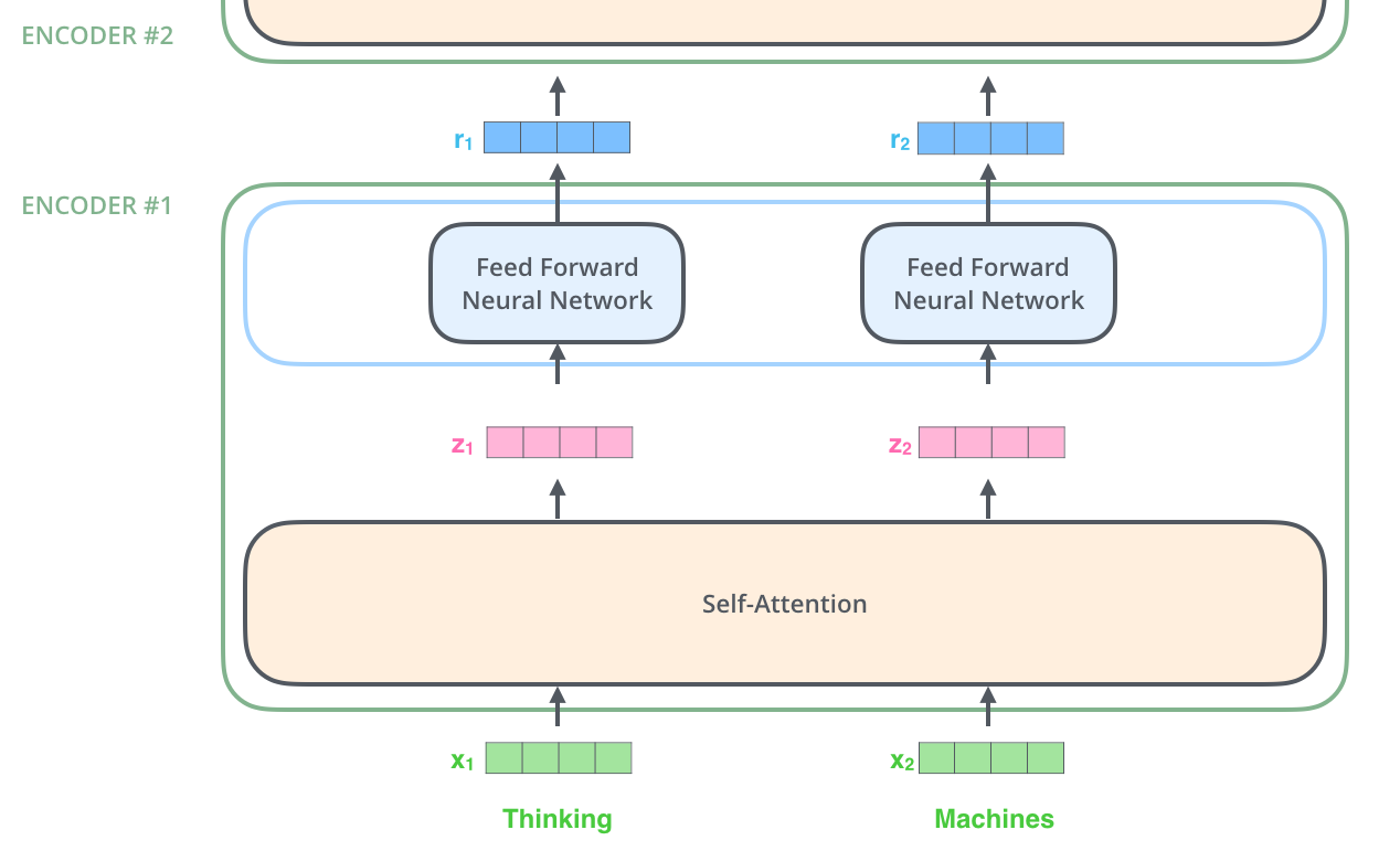
Fig. 35 Encoder Layer architecture. Image source illustrated-transformer#
Fig. 35 shows the architecture of an encoder layer. The input sequence is first converted into a sequence of vector embeddings \(X = \{x_1, x_2, ..., x_n\}\) using an embedding layer. The embeddings are then processed by the self-attention layer and then pass through a feed-forward network. The output of the feed-forward network is then added to the input embeddings to produce the output embeddings \(Y = \{y_1, y_2, ..., y_n\}\).
The encoder is composed of a stack of identical layers, all similar to the one shown in Fig. 35. The output of the encoder is the output embeddings \(Y\) of the last layer.
Decoder#
The decoder is responsible for generating the output sequence based on the information extracted by the encoder. The goal is to train a neural network that can leverage the correlations between the different elements of the input sequence to perform generative tasks such as text generation, image generation, or speech synthesis.
The input of the decoder is a sequence of elements. For example, in the case of audio, the input sequence is a sequence of frames. The sequence is first converted into a sequence of vector embeddings that are then processed by the decoder layers.
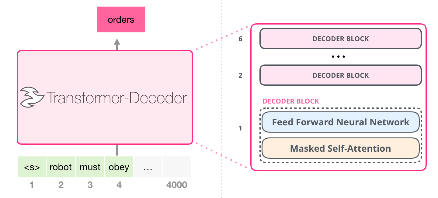
Fig. 36 Decoder Layer architecture. Image source illustrated-gpt-2#
The masked self-attention layer is similar to the self-attention layer of the encoder. The only difference is that the masked self-attention layer is masked to prevent the decoder from “seeing” the future elements of the sequence. The output is then processed by a feed-forward network. The output of the feed-forward network is then added to the input embeddings to produce the output embeddings \(Y = \{y_1, y_2, ..., y_n\}\).
When training a decoder-only model, the output embeddings \(Y\) at each position \(i\) are used to predict the next element of the sequence \(y_{i+1}\).
💡 In contrast with RNNs, the training of the decoder is autoregressive. This means that the model is trained to predict the next element of the sequence based on the previous elements of the sequence. While for RNNs we need to recursively feed the output of the model back as input, for transformers we can compute the output of the model in parallel for all the elements of the sequence.
💡 During inference, the decoder is used to generate the output sequence. However, the target is not available during inference. Instead, the output of the decoder at each position \(i\) is used as input for the next position \(i+1\). This process is repeated until a special token is generated or a maximum number of steps is reached. This is one of the reason why, the inference on transformers is slower than the training.
Encoder-Decoder#
If we combine the encoder and decoder, we get a sequence-to-sequence model. The encoder is used to extract features from the input sequence and the decoder is used to generate the output sequence based (or conditioned) on the extracted features. One example of sequence-to-sequence model is a music style transfer model. The input sequence may be a song in a specific style and the output sequence may be the same song in another style. The encoder is used to extract features from the input song and the decoder is used to generate the output song based on the extracted features.

Fig. 37 Encoder-Decoder architecture. Image source illustrated-transformer#
Fig. 37 shows the architecture of an encoder-decoder model. The input sequence is first converted into a sequence of vector embeddings \(X = \{x_1, x_2, ..., x_n\}\) using an embedding layer. The embeddings are then processed by the encoder layers. The output of the encoder is the output embeddings \(Y = \{y_1, y_2, ..., y_n\}\) of the last layer. The output embeddings are then processed by the decoder layers. Here we have an additional attention layer that allows the decoder to combine the output embeddings of the encoder with the output embeddings of the decoder. The output of the decoder is the output embeddings \(Z = \{z_1, z_2, ..., z_n\}\) of the last layer.
🖊️ The encoder-decoder attention is usually referred to as the cross-attention layer. The self-attention layer in the encoder is usually referred to as the self-attention layer. The self-attention layer in the decoder is usually referred to as the masked self-attention layer because it is masked to prevent the decoder from “seeing” the future elements of the sequence. All these layers, however, perform the same operation that we will describe in the following sections.
Transformer Components#
Fig. 38 Encoder-decoder Transformer architecture.#
We will describe the different components of the transformer architecture from bottom to top. We will follow the Fig. 34 and start with the embedding layer, then the positional encoding, the self-attention layer, and so on.
Embedding Layer#
When training a transformer model, the input sequence is first converted into a sequence of vector embeddings. Those vector embeddings are created using an embedding layer. The embedding layer is a simple linear layer that maps each element of the input sequence to a vector of a specific size. The size of the vector is called the embedding size and is a power of 2, usually between 128 and 1024. The embedding size is a hyperparameter of the model.
We can see the embedding layer as a lookup table that maps each element of the input sequence to a vector of a specific size. The embedding layer is initialized randomly and is trained through backpropagation. The embedding layer is usually the first layer of the encoder and the decoder.
Fig. 39 Embedding layer as a lookup table. Image source lena-voita#
Fig. 39 shows an example of an embedding layer in the context of NLP (it is simpler to visualize in this context). The embedding layer is a lookup table that maps each word of the input sequence to a vector of a specific size.
Positional Encoding#
After the embedding layer, the input sequence is converted into a sequence of vector embeddings. As we can see later, the attention mechanism, at the core of the transformer architecture, does not take into account the position of each element of the sequence. To inject this information into the model, we use a technique called positional encoding.
There are different implementations of positional encoding. The traditional implementation is based on sinusoidal functions. For each position \(i\) of the input sequence, we compute a vector \(PE_i\) of the same size as the embeddings. The vector \(PE_i\) is then added to the embeddings \(x_i\) to produce the final embeddings \(x_i + PE_i\).
How can we compute the vector \(PE_i\)? The vector \(PE_i\) is computed using a combination of sinusoidal functions. We define a set of frequencies \(f\) and compute the vector \(PE_i\) as follows:
where \(d\) is the size of the embeddings. The frequencies \(f\) are computed as follows:
The frequencies \(f\) are computed using a geometric progression. The first frequency is \(f_1 = 1/10000^{2 \times 1/d}\), the second frequency is \(f_2 = 1/10000^{2 \times 2/d}\), and so on. The frequencies are then used to compute the vector \(PE_i\). \(d\) is the size of the embeddings. The vector \(PE_i\) is then added to the embeddings \(x_i\) to produce the vector \(x_i + PE_i\) that will be the input of the network.
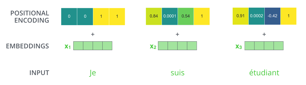
Fig. 40 Positional encoding example. Image source illustrated-transformer#
Fig. 40 shows an example of positional encoding (again in the context of NLP). Each element in a \(PE_i\) vector is computed using a sinusoidal function.
💡 The idea behind the use of sinusoidal functions is to allow the model to be able to encode regularities in the position of the elements of the sequence. Different frequencies may have similar values with different regularities. In a complete data-driven approach, the model would learn the regularities according to the patterns found in the data.
Attention Mechanism#
At this point of the chapter, we have converted the input sequence into a sequence of vector embeddings. The next step is to process the embeddings using the attention mechanism. The attention mechanism is the core of the transformer architecture. It is used to learn the relationships between the different elements of the sequence.
The attention mechanism is a mechanism that allows the model to learn the relationships between the different elements of the sequence. the process can be divided into three steps:
Query, Key, and Value. The input embeddings are first split into three vectors: the query vector, the key vector, and the value vector.
Attention. The query vector is compared to the key vector to produce a score, e.g., a float value between 0 and 1. The score is then used to compute a weighted average of the value vector. The weighted average is called the attention vector.
Output. The attention vector is then processed by a linear layer to produce the output vector.
Fig. 41 Attention mechanism steps. Image source towardsdatascience#
Fig. 41 shows an example of the attention mechanism. The input embeddings are first split into three vectors: the query vector, the key vector, and the value vector.
Query. The query vector is used to ask to all other elements of the sequence how much they are related to the current element. The dot product between the query vector and the key vector is used to compute a score (the higher the score, the more related the elements are). The score is then normalized using a softmax function to produce a probability distribution over all the elements of the sequence.
Key. The key vector is used to answer to the query. Each value vector is multiplied with the query of the other elements of the sequence. query and key are the vectors that, multiplied together, produce the score.
Value. Once obtained a score for each element of the sequence, the value vector is multiplied with the score to produce a weighted average of the value vector. The weighted average is called the attention vector.
The final vector representation for a given input element of the sequence is given by the sum of the attention vectors of all the elements of the sequence.
💡 Note that, the attention mechanism is usually referred to self-attention because the attention score is computed between a given element of the sequence and all the other elements, including itself.
If we put this into equations, we have:
where \(Q\) is the query vector, \(K\) is the key vector, \(V\) is the value vector, and \(d_k\) is the size of the key vector. \(\sqrt{d_k}\) is used to scale the dot product between \(Q\) and \(K\). The softmax function is applied to each row of the matrix \(QK^T\) to produce a probability distribution over all the elements of the sequence. The probability distribution is then used to compute a weighted average of the value vector \(V\). The formula above is the matrix form of the attention mechanism.
Each element of the sequence is processed independently by the attention mechanism. This means that the attention mechanism can be computed in parallel for all the elements of the sequence. This is one of the reasons why transformers are faster than RNNs on modern hardware (e.g., GPUs).
Coming back to our bottom-up approach, the attention mechanism is used to process the embeddings of the input sequence (after the positional encoding). The output of the attention mechanism is a sequence of vectors having the same size and shape as the input embeddings. After the attention mechanism a simple linear layer is used to produce the output embeddings (typically without altering the size of the embeddings).
Multi-head Attention. The attention mechanism described above is called single-head attention. In practice, the attention mechanism is computed multiple times in parallel on subsets of the embeddings. Each subset is called a head. Before feeding the embedding into the self-attention layer, in case of multi-head attention, the vector is first split into parts and each part is processed by a different head. The output of the self-attention layer is then the concatenation of the output of each head. The output of the self-attention layer is then processed by a linear layer to produce the output embeddings.

Fig. 42 Example of multi-head attention (e.g., number of attention heads \(h=2\)).#
Fig. 42 shows an example of multi-head attention. In practice, all implementations of modern transformer models use multi-head attention (e.g., BERT, GPT-2, ViT, etc.). The number of heads is a hyperparameter of the model, similarly to the embedding size. It is worth noting that, the number of heads should be a number such that the size of the input embedding is divisible by the number of heads. For example, if the embedding size is \(512\), we can use \(8\) heads (\(512/8 = 64\)) or \(16\) heads (\(512/16 = 32\)) but not \(10\) heads (\(512/10 = 51.2\)).
Feed-Forward and Residual Connections#
After the attention mechanism, the output embeddings are processed by a feed-forward network. The feed-forward network is a simple linear layer followed by a non-linear activation function (e.g., ReLU).
Similarly to what we have seen with ResNets [], in each layer of the encoder and decoder, there are residual connections that sum up the output of a sub-layer with the input of the sub-layer.
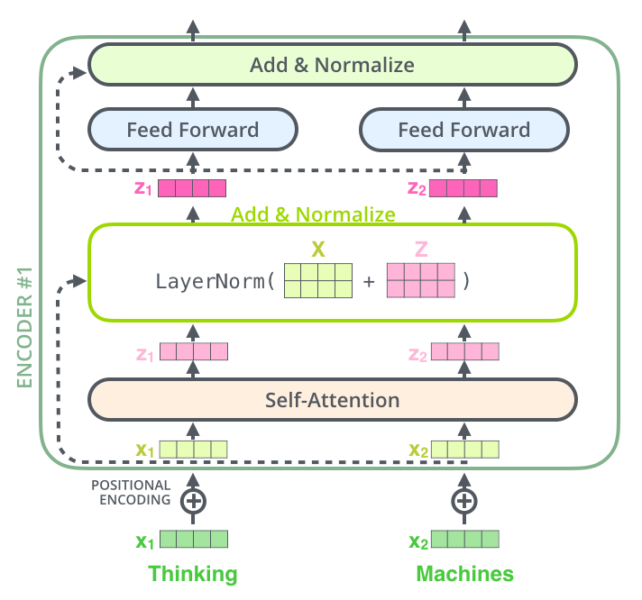
Fig. 43 Residual connections and layer normalization. Image source illustrated-transformer#
Fig. 43 shows an example of residual connections and layer normalization. Both the output of the attention layer and the output of the feed-forward network are added to the input embeddings. The output of the residual connections is then processed by a layer normalization layer. Layer normalization is a technique that consists of normalizing the output of a layer using the mean and variance of the output of the layer. Layer normalization is used to make the training of the model more stable and efficient.
Encoder and Decoder Models#
At this point we have all the ingredients to create an encoder transformer layer. The encoder model is composed of:
Embedding layer. The embedding layer converts the input sequence into a sequence of vector embeddings.
Positional encoding. The positional encoding injects information about the position of each element of the sequence into the model.
Encoder layers. The encoder layers process the embeddings using:
Multi-head attention. The multi-head attention mechanism is used to learn the relationships between the different elements of the sequence.
Feed-forward network. The feed-forward network is used to process the output of the multi-head attention mechanism.
Residual connections. The residual connections are used to sum up the output of the multi-head attention mechanism with the input embeddings.
Layer normalization. The layer normalization is used to normalize the output of the encoder layer.
A stack of encoder layers is used to create the encoder model. The output of the encoder is the output embeddings of the last encoder layer. We can use this encoder model to extract features from a sequence. For example, we can use the encoder model to extract features from an audio sequence and then use those features to perform speech recognition.
The decoder model, when used in decoder-only mode, is similar to the encoder model. The decoder model is composed of:
Embedding layer. The embedding layer converts the input sequence into a sequence of vector embeddings.
Positional encoding. The positional encoding injects information about the position of each element of the sequence into the model.
Decoder layers. The decoder layers process the embeddings using:
Masked multi-head attention. The masked multi-head attention mechanism is used to learn the relationships between the different elements of the sequence. The attention mechanism is masked to prevent the decoder from “seeing” the future elements of the sequence.
Feed-forward network. The feed-forward network is used to process the output of the multi-head attention mechanism.
Residual connections. The residual connections are used to sum up the output of the multi-head attention mechanism with the input embeddings.
Layer normalization. The layer normalization is used to normalize the output of the decoder layer.
Notice that, the attention layer of the decoder is referred as masked multi-head attention because it is masked to prevent the decoder from “seeing” the future elements of the sequence.
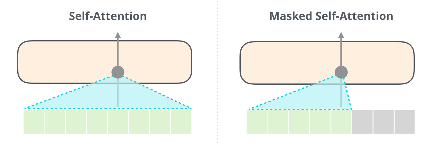
Fig. 44 Comparison between self-attention and masked self-attention. Image source illustrated-transformer#
Fig. 44 shows an example of masked self-attention and the comparison with self-attention operation. When processing element \(x_i\), the masked self-attention mechanism is masked to prevent the decoder from “seeing” the future elements of the sequence \(x_{i+1}, x_{i+2}, ..., x_n\). The masked-self attention mechanism is usually implemented by adding a mask to the softmax function. The mask contains \(-\infty\) values for all the elements of the sequence that we want to mask. The \(-\infty\) values are used to set the attention score to \(0\) after the softmax function. This means that the decoder will not be able to attend to the masked elements of the sequence.
Encoder-Decoder (Sequence-to-sequence) Models#
We have seen how to design layers for the encoder and decoder models. Encoder models are used to extract features from a sequence. Decoder models are used to generate a sequence based on the previous elements of the sequence. Encoder-decoder models are used to generate data conditioned on another sequence. For example, we can use an encoder-decoder model to translate a sentence from English to French or to generate the transcription of an audio sequence.
The encoder-decoder model is composed of:
Encoder. The encoder is used to extract features from the input sequence.
Decoder. The decoder is used to generate the output sequence based on the extracted features.
Cross-attention (encoder-decoder attention). The decoder in this case adds an additional attention layer that allows the decoder to condition the output sequence on the input sequence. The cross-attention layer is similar to the self-attention layer of the encoder. The only difference is that the cross-attention layer is used to learn the relationships between the elements of the input sequence and the elements of the output sequence.
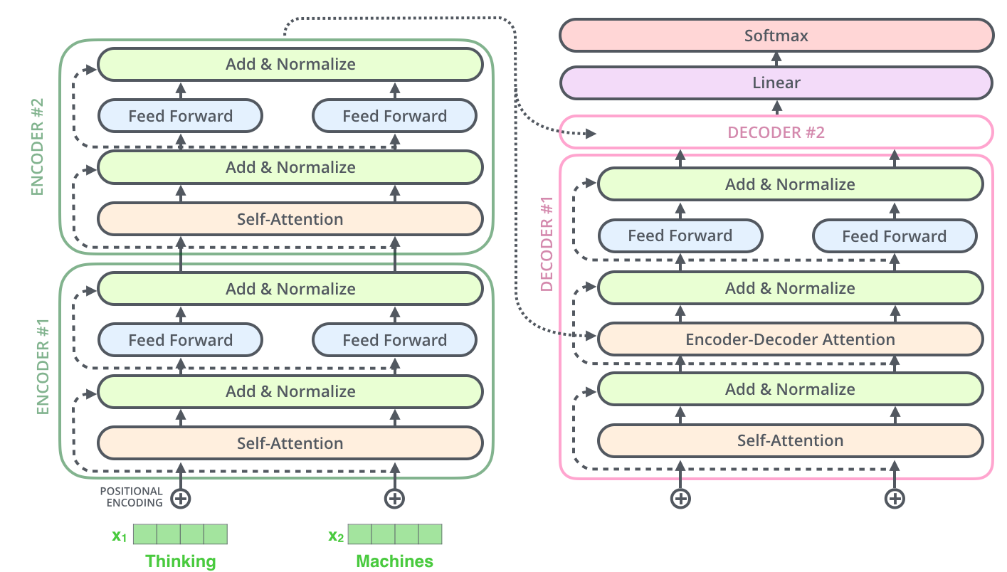
Fig. 45 Encoder-decoder model showing the cross-attention layer. Image source illustrated-transformer#
Fig. 45 shows an example of an encoder-decoder model. The input sequence is first converted into a sequence of vector embeddings \(X = \{x_1, x_2, ..., x_n\}\) using an embedding layer. The embeddings are then processed by the encoder layers. The output of the encoder is the output embeddings \(Y = \{y_1, y_2, ..., y_n\}\) of the last layer. The output embeddings are then processed by the decoder layers. Here we have an additional attention layer that leverage key and value vectors from the encoder to combine the output embeddings of the encoder with the output embeddings of the decoder. The output of the decoder is the output embeddings \(Z = \{z_1, z_2, ..., z_n\}\) of the last layer. The example reported in Fig. 45 is in the context of NLP. However, the very same architecture can be used in the context of audio, images, or multi-modal data (e.g., an audio sequence is encoded into a sequence of embeddings and then decoded into a sequence of text for speech recognition) [RKX+23].
An Encoder-Decoder Model in PyTorch#
We have seen how to design the different components of the transformer architecture. In this section, we will see how to implement an encoder-decoder model in pure PyTorch.
Embedding Layer#
The embedding layer is a simple linear layer that maps each element of the input sequence to a vector of a specific size. The size of the vector is called the embedding size and is (for convenience) a power of 2, or at least divisible by 2 and 3.
import torch.nn as nn

class EmbeddingLayer(nn.Module):
    def __init__(self, vocab_size, embedding_size):
        super().__init__()
        self.embedding = nn.Embedding(vocab_size, embedding_size)

    def forward(self, x):
        return self.embedding(x)
When calling the embedding layer, we pass the input sequence in terms of ids. The ids are integers that represent the elements of the sequence. For example, in the case of text, the ids are the indices of the words in the vocabulary. In the case of audio, the ids are the indices of the frames in the vocabulary. Depending on the domain, we may not need an embedding layer. For example, in the case of images, we can use the pixel values as input to the model.
Let’s take a look at the input-output shape of the embedding layer.
Input. The input of the embedding layer is a sequence of ids. The shape of the input is \((B, S)\) where \(B\) is the batch size and \(S\) is the sequence length.
Output. The output of the embedding layer is a sequence of vector embeddings. The shape of the output is \((B, S, E)\) where \(B\) is the batch size, \(S\) is the sequence length, and \(E\) is the embedding size.
Positional Encoding#
The positional encoding is a technique that consists of injecting information about the position of each element of the sequence into the model. There are different implementations of positional encoding. The traditional implementation is based on sinusoidal functions. For each position \(i\) of the input sequence, we compute a vector \(PE_i\) of the same size as the embeddings. The vector \(PE_i\) is then added to the embeddings \(x_i\) to produce the final embeddings \(x_i + PE_i\).
import torch
import torch.nn as nn

class PositionalEncoding(nn.Module):
    def __init__(self, embedding_size, dropout=0.1, max_len=5000):
        super().__init__()
        self.dropout = nn.Dropout(p=dropout)

        pe = torch.zeros(max_len, embedding_size)
        position = torch.arange(0, max_len, dtype=torch.float).unsqueeze(1)
        div_term = torch.exp(torch.arange(0, embedding_size, 2).float() * (-math.log(10000.0) / embedding_size))
        pe[:, 0::2] = torch.sin(position * div_term)
        pe[:, 1::2] = torch.cos(position * div_term)
        pe = pe.unsqueeze(0).transpose(0, 1)
        self.register_buffer('pe', pe)

    def forward(self, x):
        x = x + self.pe[:x.size(0), :]
        return self.dropout(x)
The positional encoding is implemented as a PyTorch module. It is initialized with the embedding size and the dropout rate. The positional encoding is computed in the forward method. We define a set of frequencies \(f\) and compute the vector \(PE_i\) accordingly (review the Section on Positional Encoding for more details).
When passing through the positional encoding layer, the input embeddings are summed up with the positional encoding vectors, therefore their shape does not change $\((B, S, E) \rightarrow (B, S, E)\)$.
There are several other implementations of positional encoding. For example, we can have a learnable positional encoding that is learned during training. It is implemented using an embedding layer.
import torch
import torch.nn as nn

class PositionalEncoding(nn.Module):
    def __init__(self, embedding_size, dropout=0.1, max_len=5000):
        super().__init__()
        self.dropout = nn.Dropout(p=dropout)
        self.embedding = nn.Embedding(max_len, embedding_size)

    def forward(self, x):
        position = torch.arange(0, x.size(1), dtype=torch.long, device=x.device)
        position = position.unsqueeze(0).expand_as(x)
        x = x + self.embedding(position)
        return self.dropout(x)
In this case, the positional encoding is learned during training. We should pay attention to the fact that this implementation does not force the model to learn the time-related patterns in the data. The name positional encoding is only used for convenience as it may learn other patterns in the data.
Attention Mechanism#
Diving inside the transformer architecture, we need to implement the attention mechanism. The attention mechanism is a mechanism that allows the model to learn the relationships between the different elements of the sequence. The process can be divided into three steps:
Query, Key, and Value. The input embeddings are first split into three vectors: the query vector, the key vector, and the value vector.
Attention. The query vector is compared to the key vector to produce a score, e.g., a float value between 0 and 1. The score is then used to compute a weighted average of the value vector. The weighted average is called the attention vector.
Output. The attention vector is then processed by a linear layer to produce the output vector.
import torch
import torch.nn as nn

class MHSA(nn.Module):
    def __init__(self, embedding_size, num_heads):
        super().__init__()
        self.num_heads = num_heads
        self.head_size = embedding_size // num_heads
        self.scale = self.head_size ** -0.5

        self.query = nn.Linear(embedding_size, embedding_size)
        self.key = nn.Linear(embedding_size, embedding_size)
        self.value = nn.Linear(embedding_size, embedding_size)
        self.out = nn.Linear(embedding_size, embedding_size)

    def forward(self, x):
        B, S, E = x.size()
        Q = self.query(x).view(B, S, self.num_heads, self.head_size).transpose(1, 2)
        K = self.key(x).view(B, S, self.num_heads, self.head_size).transpose(1, 2)
        V = self.value(x).view(B, S, self.num_heads, self.head_size).transpose(1, 2)

        scores = torch.matmul(Q, K.transpose(-2, -1)) * self.scale
        scores = scores.softmax(dim=-1)
        scores = scores.matmul(V).transpose(1, 2).reshape(B, S, E)
        return self.out(scores)
The class MHSA implements the multi-head attention mechanism. The input of the attention mechanism is a sequence of embeddings. The embeddings are first split into three vectors: the query vector, the key vector, and the value vector. The query, key, and value vectors are then processed by three linear layers. The output of the linear layers is then split into multiple heads. The number of heads is a hyperparameter of the model. The output of the attention mechanism is the concatenation of the output of each head. The output of the attention mechanism is then processed by a linear layer to produce the output embeddings.
Similarly to the positional encoding, the MHSA is implemented as a PyTorch module. The input and output of the MHSA are embeddings, therefore their shape does not change $\((B, S, E) \rightarrow (B, S, E)\)$.
Test MHSA implementation
We can test the implementation of the MHSA module by creating a random input tensor and passing it through the module.
import torch
from mhsa import MHSA # import the MHSA module

mhsa = MHSA(embedding_size=512, num_heads=8) # create the MHSA module
x = torch.randn(2, 10, 512) # create a random input tensor
y = mhsa(x) # pass the input tensor through the MHSA module
print(y.shape) # print the shape of the output tensor
Cross-Attention#
The cross-attention layer is similar to the self-attention layer of the encoder. The only difference is that the cross-attention layer is used to learn the relationships between the elements of the input sequence and the elements of the output sequence.
import torch
import torch.nn as nn

class CrossAttention(nn.Module):
    def __init__(self, embedding_size, num_heads):
        super().__init__()
        self.num_heads = num_heads
        self.head_size = embedding_size // num_heads
        self.scale = self.head_size ** -0.5

        self.query = nn.Linear(embedding_size, embedding_size)
        self.key = nn.Linear(embedding_size, embedding_size)
        self.value = nn.Linear(embedding_size, embedding_size)
        self.out = nn.Linear(embedding_size, embedding_size)

    def forward(self, x, y):
        '''
        x: input embeddings
        y: vector to "cross-attend" to
        '''
        B, S, E = x.size()
        Q = self.query(x).view(B, S, self.num_heads, self.head_size).transpose(1, 2) # queries are computed from x
        K = self.key(y).view(B, S, self.num_heads, self.head_size).transpose(1, 2) # keys are computed from y
        V = self.value(y).view(B, S, self.num_heads, self.head_size).transpose(1, 2) # values are computed from y

        scores = torch.matmul(Q, K.transpose(-2, -1)) * self.scale
        scores = scores.softmax(dim=-1)
        scores = scores.matmul(V).transpose(1, 2).reshape(B, S, E)
        return self.out(scores)
As noted also in code comments, the queries are computed from the input embeddings \(x\) while the keys and values are computed from the vector \(y\). All the other considerations are the same as the self-attention layer (e.g., the output of the cross-attention layer is the concatenation of the output of each head).
Feed-Forward and Residual Connections#
After the attention mechanism, the output embeddings are processed by a feed-forward network. The feed-forward network is a simple linear layer followed by a non-linear activation function (e.g., ReLU).
Similarly to what we have seen with ResNets [], in each layer of the encoder and decoder, there are residual connections that sum up the output of a sub-layer with the input of the sub-layer.
import torch
import torch.nn as nn

class FeedForward(nn.Module):
    def __init__(self, embedding_size, hidden_size):
        super().__init__()
        self.linear1 = nn.Linear(embedding_size, hidden_size)
        self.linear2 = nn.Linear(hidden_size, embedding_size)
        self.relu = nn.ReLU()

    def forward(self, x):
        x = self.relu(self.linear1(x))
        x = self.linear2(x)
        return x

class Residual(nn.Module):
    def __init__(self, sublayer, dropout):
        super().__init__()
        self.sublayer = sublayer
        self.dropout = nn.Dropout(p=dropout)
        self.norm = nn.LayerNorm(sublayer.size)

    def forward(self, x):
        return x + self.dropout(self.sublayer(self.norm(x)))
The class FeedForward implements the feed-forward network. The class Residual implements the residual connections. The Residual class is usually not used in real implementations of transformer models.
Instead, the residual connections are implemented directly in the encoder and decoder layers.
# ... other code ...
x # is the tensor we want to add for the residual connection
x_ff = self.ff(x) # pass x through the feed-forward network
x_ff = self.dropout(x_ff) # apply dropout
x = x + x_ff # add the residual connection
Encoder and Decoder Models#
At this point we have all the ingredients to create an encoder transformer layer. The encoder model is composed of:
Embedding layer. The embedding layer converts the input sequence into a sequence of vector embeddings. If we deal with vectorized data (e.g., images), we can skip this step or implement it differently [LYC+20].
Positional encoding. The positional encoding injects information about the position of each element of the sequence into the model.
Encoder layers. The encoder layers process the embeddings using:
Multi-head attention. The multi-head attention mechanism is used to learn the relationships between the different elements of the sequence.
Feed-forward network. The feed-forward network is used to process the output of the multi-head attention mechanism.
Residual connections. The residual connections are used to sum up the output of the multi-head attention mechanism with the input embeddings.
Layer normalization. The layer normalization is used to normalize the output of the encoder layer.
Output. The output of the encoder is the output embeddings of the last encoder layer.
A stack of encoder layers is used to create the encoder model. The output of the encoder is the output embeddings of the last encoder layer.
import torch
import torch.nn as nn

class EncoderLayer(nn.Module):
    def __init__(self, embedding_size, num_heads, hidden_size, dropout):
        super().__init__()
        self.mhsa = MHSA(embedding_size, num_heads)
        self.ff = FeedForward(embedding_size, hidden_size)
        self.residual1 = Residual(self.mhsa, dropout)
        self.residual2 = Residual(self.ff, dropout)

    def forward(self, x):
        x = self.residual1(x)
        x = self.residual2(x)
        return x

class Encoder(nn.Module):
    def __init__(self, embedding_size, num_heads, hidden_size, dropout, num_layers):
        super().__init__()
        self.layers = nn.ModuleList([EncoderLayer(embedding_size, num_heads, hidden_size, dropout) for _ in range(num_layers)])
        self.norm = nn.LayerNorm(embedding_size)

    def forward(self, x):
        for layer in self.layers:
            x = layer(x)
        return self.norm(x)
The class EncoderLayer implements a single encoder layer. The class Encoder implements a stack of encoder layers. The output of the encoder is the output embeddings of the last encoder layer.
Note on the number of layers
The number of layers is a hyperparameter of the model. The number of layers is usually between 6 and 12. The number of layers is usually the same for the encoder and decoder. However, it is possible to use a different number of layers for the encoder and decoder.
Conclusion#
In this chapter, we have seen all the components behind one of the most popular deep learning architectures: the transformer (encoder decoder) and its encoder-only and decoder-only variants. We have seen how to implement the different components of the transformer architecture in pure PyTorch.
This architecture has basically revolutionized the field of deep learning. It has been used in many different domains (e.g., NLP, audio, images, multi-modal data, etc.) and has achieved state-of-the-art results in many different tasks (e.g., speech recognition, machine translation, image classification, etc.).
In the next chapter, we will get our hands dirty and we will see how to use the transformer architecture in practice, both starting from scratch and using pre-trained models.